Multiple-View Object Recognition in Band-Limited Distributed Camera - PowerPoint PPT Presentation

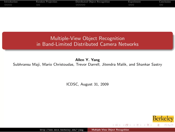
Introduction Random Projection Distributed Object Recognition Experiment Conclusion Multiple-View Object Recognition in Band-Limited Distributed Camera Networks Allen Y. Yang Subhransu Maji, Mario Christoudas, Trevor Darrell, Jitendra Malik, and Shankar Sastry ICDSC, August 31, 2009 Multiple-View Object Recognition http://www.eecs.berkeley.edu/~yang

Introduction Random Projection Distributed Object Recognition Experiment Conclusion Motivation: Object Recognition Affine invariant features, SIFT. SIFT Feature Matching [Lowe 1999, van Gool 2004] (a) Autostitch (b) Recognition Bag of Words [Nister 2006] Multiple-View Object Recognition http://www.eecs.berkeley.edu/~yang

Introduction Random Projection Distributed Object Recognition Experiment Conclusion Object Recognition in Band-Limited Sensor Networks Compress scalable SIFT tree [Girod et al. 2009] 1 Multiple-view SIFT feature selection [Darrell et al. 2008] 2 Multiple-View Object Recognition http://www.eecs.berkeley.edu/~yang

Introduction Random Projection Distributed Object Recognition Experiment Conclusion Problem Statement L camera sensors observe a single object in 3-D. 1 The mutual information between cameras are unknown, cross-sensor communication is 2 prohibited. On each camera, seek an encoding function for a nonnegative, sparse histogram x i 3 f : x i ∈ R D �→ y i ∈ R d On the base station, upon receiving y 1 , y 2 , · · · , y L , simultaneously recover 4 x 1 , x 2 , · · · , x L , and classify the object class in space. Multiple-View Object Recognition http://www.eecs.berkeley.edu/~yang

Introduction Random Projection Distributed Object Recognition Experiment Conclusion Key Observations (a) Histogram 1 (b) Histogram 2 All histograms are nonnegative and sparse . Multiple-view histograms share joint sparse patterns . Classification is based on the similarity measure in ℓ 2 -norm (linear kernel) or ℓ 1 -norm (intersection kernel). Multiple-View Object Recognition http://www.eecs.berkeley.edu/~yang

Introduction Random Projection Distributed Object Recognition Experiment Conclusion Compress SIFT Histograms: Random Projection y = A x Coefficients of A ∈ R d × D are drawn from zero-mean Gaussian distribution. Johnson-Lindenstrauss Lemma [Johnson & Lindenstrauss 1984, Frankl 1988] For n number of point cloud in R D , given distortion threshold ǫ , for any d > O ( ǫ 2 log n ) , a Gaussian random projection f ( x ) = A x ∈ R d preserves pairwise ℓ 2 -distance (1 − ǫ ) � x i − x j � 2 2 ≤ � f ( x i ) − f ( x j ) � 2 2 ≤ (1 + ǫ ) � x i − x j � 2 2 . Multiple-View Object Recognition http://www.eecs.berkeley.edu/~yang

Introduction Random Projection Distributed Object Recognition Experiment Conclusion From J-L Lemma to Compressive Sensing (a) J-L lemma (b) Compressive sensing Problem I: J-L lemma does not provide means to reconstruct histogram hierarchy . 1 Problem II: Gaussian projection does not preserve ℓ 1 -distance (for intersection kernels). 2 Problem III: Difficult (if not impossible) to incorporate multiple-view information. 3 Multiple-View Object Recognition http://www.eecs.berkeley.edu/~yang

Introduction Random Projection Distributed Object Recognition Experiment Conclusion From J-L Lemma to Compressive Sensing (a) J-L lemma (b) Compressive sensing Problem I: J-L lemma does not provide means to reconstruct histogram hierarchy . 1 Problem II: Gaussian projection does not preserve ℓ 1 -distance (for intersection kernels). 2 Problem III: Difficult (if not impossible) to incorporate multiple-view information. 3 Compressive sensing provides principled solutions to the above problems. Multiple-View Object Recognition http://www.eecs.berkeley.edu/~yang

Introduction Random Projection Distributed Object Recognition Experiment Conclusion Compressive Sensing Noise-free case Assume x 0 is sufficiently k -sparse and mild condition on A , ( P 1 ) : min � x � 1 subject to y = A x recovers the exact solution. Multiple-View Object Recognition http://www.eecs.berkeley.edu/~yang

Introduction Random Projection Distributed Object Recognition Experiment Conclusion Compressive Sensing Noise-free case Assume x 0 is sufficiently k -sparse and mild condition on A , ( P 1 ) : min � x � 1 subject to y = A x recovers the exact solution. Matching Pursuit [Mallat-Zhang 1993] Initialization: 1 y a 1 y = [ A ; − A ]˜ x , where ˜ x ≥ 0 a 2 x ← 0; r 0 ← y ; Sparse support I = ∅ a 3 k ← 0; ˜ − a 3 − a 2 − a 1 Multiple-View Object Recognition http://www.eecs.berkeley.edu/~yang

Introduction Random Projection Distributed Object Recognition Experiment Conclusion Compressive Sensing Noise-free case Assume x 0 is sufficiently k -sparse and mild condition on A , ( P 1 ) : min � x � 1 subject to y = A x recovers the exact solution. Matching Pursuit [Mallat-Zhang 1993] Initialization: 1 y a 1 y = [ A ; − A ]˜ x , where ˜ x ≥ 0 a 2 x ← 0; r 0 ← y ; Sparse support I = ∅ a 3 k ← 0; ˜ − a 3 k ← k + 1: 2 − a 2 r 1 − a 1 y i = arg max j �∈I { a T j r k − 1 } x 1 a 1 a 1 a 2 Update : I = I ∪ { i } ; x i = a T i r k − 1 ; a 3 r k = r k − 1 − x i a i x 3 a 3 − a 3 − a 2 − a 1 Multiple-View Object Recognition http://www.eecs.berkeley.edu/~yang

Introduction Random Projection Distributed Object Recognition Experiment Conclusion Compressive Sensing Noise-free case Assume x 0 is sufficiently k -sparse and mild condition on A , ( P 1 ) : min � x � 1 subject to y = A x recovers the exact solution. Matching Pursuit [Mallat-Zhang 1993] Initialization: 1 y a 1 y = [ A ; − A ]˜ x , where ˜ x ≥ 0 a 2 x ← 0; r 0 ← y ; Sparse support I = ∅ a 3 k ← 0; ˜ − a 3 k ← k + 1: 2 − a 2 r 1 − a 1 y i = arg max j �∈I { a T j r k − 1 } x 1 a 1 a 1 a 2 Update : I = I ∪ { i } ; x i = a T i r k − 1 ; a 3 r k = r k − 1 − x i a i x 3 a 3 − a 3 − a 2 − a 1 If : � r k � 2 > ǫ , go to STEP 2; 3 Else : output ˜ x Multiple-View Object Recognition http://www.eecs.berkeley.edu/~yang

Introduction Random Projection Distributed Object Recognition Experiment Conclusion Other Fast ℓ 1 -Min Routines Homotopy Methods: 1 Polytope Faces Pursuit (PFP) [Plumbley 2006] Least Angle Regression (LARS) [Efron-Hastie-Johnstone-Tibshirani 2004] Gradient Projection Methods 2 Gradient Projection Sparse Representation (GPSR) [Figueiredo-Nowak-Wright 2007] Truncated Newton Interior-Point Method (TNIPM) [Kim-Koh-Lustig-Boyd-Gorinevsky 2007] Iterative Thresholding Methods 3 Soft Thresholding [Donoho 1995] Sparse Reconstruction by Separable Approximation (SpaRSA) [Wright-Nowak-Figueiredo 2008] Proximal Gradient Methods [Nesterov 1983, Nesterov 2007] 4 FISTA [Beck-Teboulle 2009] Nesterov’s Method (NESTA) [Becker-Bobin-Cand´ es 2009] MATLAB Toolboxes SparseLab: http://sparselab.stanford.edu/ ℓ 1 Homotopy: http://users.ece.gatech.edu/~sasif/homotopy/index.html SpaRSA: http://www.lx.it.pt/~mtf/SpaRSA/ Multiple-View Object Recognition http://www.eecs.berkeley.edu/~yang

Introduction Random Projection Distributed Object Recognition Experiment Conclusion Distributed Object Recognition in Smart Camera Networks Outlines: How to enforce nonnegativity to decode SIFT histograms? 1 How to enforce joint sparsity across multiple camera views? 2 Multiple-View Object Recognition http://www.eecs.berkeley.edu/~yang

Introduction Random Projection Distributed Object Recognition Experiment Conclusion Enforcing Nonnegativity Polytope Pursuit Algorithms (MP, PFP, LARS): Algebraically: Do not add antipodal vertexes 1 y = [ A ; -A ]˜ x Geometrically: Pursuit on positive faces 2 a 2 x 1 a 1 c 2 x 2 a 2 a 3 Interior-Point Algorithms (Homotopy, SpaRSA): Remove any sparse support that have negative coefficients. Multiple-View Object Recognition http://www.eecs.berkeley.edu/~yang

Introduction Random Projection Distributed Object Recognition Experiment Conclusion Sparse Innovation Model Definition (SIM): ˜ x 1 = x + z 1 , . . . ˜ x L = x + z L . ˜ x is called the joint sparse component, and z i is called an innovation . Multiple-View Object Recognition http://www.eecs.berkeley.edu/~yang

Introduction Random Projection Distributed Object Recognition Experiment Conclusion Sparse Innovation Model Definition (SIM): ˜ x 1 = x + z 1 , . . . ˜ x L = x + z L . ˜ x is called the joint sparse component, and z i is called an innovation . Joint recovery of SIM ˜ 2 x 3 y 1 2 3 2 A 1 A 1 0 ··· 0 3 z 1 . . ... ... . = . . 6 7 4 . 5 4 5 . . 4 5 . y L A L 0 ··· 0 A L z L A ′ x ′ ∈ R dL . y ′ ⇔ = New histogram vector is nonnegative and sparse . 1 x is automatically determined by ℓ 1 -min: No prior training, no assumption about fixing Joint sparsity ˜ 2 cameras. Multiple-View Object Recognition http://www.eecs.berkeley.edu/~yang

Introduction Random Projection Distributed Object Recognition Experiment Conclusion CITRIC: Wireless Smart Camera Platform Available library functions CITRIC platform Full support Intel IPP Library and OpenCV . 1 JPEG compression : 10 fps. 2 3 Edge detector : 3 fps. 4 Background Subtraction : 5 fps. 5 SIFT detector : 10 sec per frame. Academic users: Multiple-View Object Recognition http://www.eecs.berkeley.edu/~yang