MSc in Computer Engineering, Cybersecurity and Artificial - PowerPoint PPT Presentation
MSc in Computer Engineering, Cybersecurity and Artificial Intelligence Course FDE , a.a. 2019/2020, Lecture 16 Review of stochastic processes and systems Prof. Mauro Franceschelli Dept. of Electrical and Electronic Engineering University of
MSc in Computer Engineering, Cybersecurity and Artificial Intelligence Course FDE , a.a. 2019/2020, Lecture 16 Review of stochastic processes and systems Prof. Mauro Franceschelli Dept. of Electrical and Electronic Engineering University of Cagliari, Italy Thursday, 7th May 2020 1 / 28
Outline Modeling measurement and process noise Brief review of stochastic models Noise model 2 / 28
Modeling measurement and process noise Introduction • So far, we have introduced the concept of measurement noise as an issue to take care in the control system and state observer design problem without a formal characterization • Sensing and actuation equipment are inevitably affected by noise, uncertainty and small modeling inaccuracies. • These issues can not be eliminated in practice but their existence can be formally characterized and taken care of during the design process. • In particular, we ask the question: can we reduce the effect of measurement and process noise on state estimation errors? 3 / 28
Modeling measurement and process noise Introduction • So far, we have introduced the concept of measurement noise as an issue to take care in the control system and state observer design problem without a formal characterization • Sensing and actuation equipment are inevitably affected by noise, uncertainty and small modeling inaccuracies. • These issues can not be eliminated in practice but their existence can be formally characterized and taken care of during the design process. • In particular, we ask the question: can we reduce the effect of measurement and process noise on state estimation errors? 3 / 28
Modeling measurement and process noise Introduction • So far, we have introduced the concept of measurement noise as an issue to take care in the control system and state observer design problem without a formal characterization • Sensing and actuation equipment are inevitably affected by noise, uncertainty and small modeling inaccuracies. • These issues can not be eliminated in practice but their existence can be formally characterized and taken care of during the design process. • In particular, we ask the question: can we reduce the effect of measurement and process noise on state estimation errors? 3 / 28
Modeling measurement and process noise Introduction • So far, we have introduced the concept of measurement noise as an issue to take care in the control system and state observer design problem without a formal characterization • Sensing and actuation equipment are inevitably affected by noise, uncertainty and small modeling inaccuracies. • These issues can not be eliminated in practice but their existence can be formally characterized and taken care of during the design process. • In particular, we ask the question: can we reduce the effect of measurement and process noise on state estimation errors? 3 / 28
Modeling measurement and process noise Measurement and process noise Our objective is to study a state estimation problem for the next discrete-time, time-varying, linear system: ① ( k + 1) = ❆ ( k ) ① ( k ) + ❇ ( k ) ✉ ( k ) + ✇ ( k ) ② ( k ) = ❈ ( k ) ① ( k ) + ✈ ( k ) where ❆ ( k ) is an n × n matrix; ❇ ( k ) is an n × r matrix; ❈ ( k ) is an n × p matrix; • The dependence of matrix A , B , C on the discrete time k could be inherent to the model or be due to the linearization of a nonlinear model at time k around the current state ① ( k ). 4 / 28
Modeling measurement and process noise Measurement and process noise ① ( k + 1) = ❆ ( k ) ① ( k ) + ❇ ( k ) ✉ ( k ) + ✇ ( k ) ② ( k ) = ❈ ( k ) ① ( k ) + ✈ ( k ) • ✇ ( k ) is an n element vector which represents process noise, i.e., an element of uncertainty in the update of the state variables to external factors or modeling inaccuracies of the dynamical system (the process). Process noise could also model actuation noise if ✇ ( k ) = ❇ ˆ ✇ ( k ) without lack of generality. • ✈ ( k ) is a p element vector which represents measurement noise, i.e., an element of unavoidable uncertainty in measurement of the system outputs by the sensing equipment. 5 / 28
Modeling measurement and process noise Measurement and process noise ① ( k + 1) = ❆ ( k ) ① ( k ) + ❇ ( k ) ✉ ( k ) + ✇ ( k ) ② ( k ) = ❈ ( k ) ① ( k ) + ✈ ( k ) • Both ✇ and ✈ are stochastic processes • If we fix the time k then ✇ ( k ) and ✈ ( k ) are vectors whose elements are random variables. 6 / 28
Modeling measurement and process noise Measurement and process noise ① ( k + 1) = ❆ ( k ) ① ( k ) + ❇ ( k ) ✉ ( k ) + ✇ ( k ) ② ( k ) = ❈ ( k ) ① ( k ) + ✈ ( k ) • Both ✇ and ✈ are stochastic processes • If we fix the time k then ✇ ( k ) and ✈ ( k ) are vectors whose elements are random variables. 6 / 28
Outline Modeling measurement and process noise Brief Review of stochastic models Noise model 7 / 28
Brief review of stochastic models Random variable • A discrete random variable X (variabile aleatoria) takes a random value among a discrete set of possible values according to a probability distribution. • For instance, the discrete random variable representing the outcome of a dice throw has possible values S = { 1 , 2 , 3 , 4 , 5 , 6] } . • Let p ( X = x ) with x ∈ S , also simply denoted as p ( x ) be the probability distribution of the discrete random variable X . • In the case of the dice, p (1) = 1 / 6, p (2) = 1 / 6, p (3) = 1 / 6, p (4) = 1 / 6, p (5) = 1 / 6, p (6) = 1 / 6 and p ( x ) = 0 for x �∈ S . Throwing the dice is called a realization of the random variable, or its outcome. 8 / 28
Brief review of stochastic models Random variable • A discrete random variable X (variabile aleatoria) takes a random value among a discrete set of possible values according to a probability distribution. • For instance, the discrete random variable representing the outcome of a dice throw has possible values S = { 1 , 2 , 3 , 4 , 5 , 6] } . • Let p ( X = x ) with x ∈ S , also simply denoted as p ( x ) be the probability distribution of the discrete random variable X . • In the case of the dice, p (1) = 1 / 6, p (2) = 1 / 6, p (3) = 1 / 6, p (4) = 1 / 6, p (5) = 1 / 6, p (6) = 1 / 6 and p ( x ) = 0 for x �∈ S . Throwing the dice is called a realization of the random variable, or its outcome. 8 / 28
Brief review of stochastic models Random variable • A discrete random variable X (variabile aleatoria) takes a random value among a discrete set of possible values according to a probability distribution. • For instance, the discrete random variable representing the outcome of a dice throw has possible values S = { 1 , 2 , 3 , 4 , 5 , 6] } . • Let p ( X = x ) with x ∈ S , also simply denoted as p ( x ) be the probability distribution of the discrete random variable X . • In the case of the dice, p (1) = 1 / 6, p (2) = 1 / 6, p (3) = 1 / 6, p (4) = 1 / 6, p (5) = 1 / 6, p (6) = 1 / 6 and p ( x ) = 0 for x �∈ S . Throwing the dice is called a realization of the random variable, or its outcome. 8 / 28
Brief review of stochastic models Random variable • A discrete random variable X (variabile aleatoria) takes a random value among a discrete set of possible values according to a probability distribution. • For instance, the discrete random variable representing the outcome of a dice throw has possible values S = { 1 , 2 , 3 , 4 , 5 , 6] } . • Let p ( X = x ) with x ∈ S , also simply denoted as p ( x ) be the probability distribution of the discrete random variable X . • In the case of the dice, p (1) = 1 / 6, p (2) = 1 / 6, p (3) = 1 / 6, p (4) = 1 / 6, p (5) = 1 / 6, p (6) = 1 / 6 and p ( x ) = 0 for x �∈ S . Throwing the dice is called a realization of the random variable, or its outcome. 8 / 28
Brief review of stochastic models Continuous random variable • A continuous random variable X takes a random value within a given continuous interval of admissible values according to a probability distribution. • Let X take values in a continuous interval [ x 1 , x 2 ] where x 1 , x 2 ∈ R • Let p ( X = x ) with x ∈ R , also simply denoted as p ( x ) be the probability density function of the random variable X 9 / 28
Brief review of stochastic models Continuous random variable • A continuous random variable X takes a random value within a given continuous interval of admissible values according to a probability distribution. • Let X take values in a continuous interval [ x 1 , x 2 ] where x 1 , x 2 ∈ R • Let p ( X = x ) with x ∈ R , also simply denoted as p ( x ) be the probability density function of the random variable X 9 / 28
Brief review of stochastic models Continuous random variable • A continuous random variable X takes a random value within a given continuous interval of admissible values according to a probability distribution. • Let X take values in a continuous interval [ x 1 , x 2 ] where x 1 , x 2 ∈ R • Let p ( X = x ) with x ∈ R , also simply denoted as p ( x ) be the probability density function of the random variable X 9 / 28
Brief review of stochastic models Continuous random variable • The probability that a given realization of the random variable belongs to an interval [ a , b ] is � b Pr ( X ∈ ( a , b )) = p ( x ) dx a � ∞ • Clearly, Pr ( X ∈ ( −∞ , ∞ )) = −∞ p ( x ) dx = 1 10 / 28
Recommend
More recommend
Explore More Topics
Stay informed with curated content and fresh updates.


