Model fitting and inference for infectious disease dynamics Useful R - - PDF document

Model fitting and inference for infectious disease dynamics Useful R commands

Contents

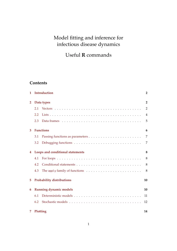
1 Introduction 2 2 Data types 2 2.1 Vectors . . . . . . . . . . . . . . . . . . . . . . . . . . . . . . . . . . . . 2 2.2 Lists . . . . . . . . . . . . . . . . . . . . . . . . . . . . . . . . . . . . . . 4 2.3 Data frames . . . . . . . . . . . . . . . . . . . . . . . . . . . . . . . . . 5 3 Functions 6 3.1 Passing functions as parameters . . . . . . . . . . . . . . . . . . . . . . 7 3.2 Debugging functions . . . . . . . . . . . . . . . . . . . . . . . . . . . . 7 4 Loops and conditional statements 8 4.1 For loops . . . . . . . . . . . . . . . . . . . . . . . . . . . . . . . . . . . 8 4.2 Conditional statements . . . . . . . . . . . . . . . . . . . . . . . . . . . 8 4.3 The apply family of functions . . . . . . . . . . . . . . . . . . . . . . . 8 5 Probability distributions 10 6 Running dynamic models 10 6.1 Deterministic models . . . . . . . . . . . . . . . . . . . . . . . . . . . . 11 6.2 Stochastic models . . . . . . . . . . . . . . . . . . . . . . . . . . . . . . 12 7 Plotting 14 1

1 Introduction

This document provides a summary of R commands that will be useful to learn or refresh in preparation for the course on Model fitting and inference for infectious disease dynamics, 16-19 June at the London School of Hygiene & Tropical Medicine. While we expect that you will have some knowledge of R, the commands listed below are the ones that we think it would be most useful for you to familiarise yourselves with in order to be able to read the code we will provide for the practical session, and to debug any code you write yourselves during the sessions. There are links in various places which will take you to web sites that provide further information, if you would like more detail on any particular concept. A good general and detailed introduction to R is provided in the R manual. Any line in R that starts with a hash (#) is interpreted as a comment and not evaluated:

# this line does nothing

For the course, please try and make sure you are running at least version 3.2.0

• f R. You can find out which R version you are running by typing

R.Version()$version.string [1] ”R version 3.2.0 (2015-04-16)”

in an R session. If your version is smaller than 3.2.0, please update to at least version 3.2.0 following the instructions on the CRAN website.

2 Data types

The data types we will be working with in the course are (named) vectors, lists, and data frames. More information on data types in R can be found in many places on the web, for example the R programming wikibook.

2.1 Vectors

Vectors are an ordered collection of simple elements such as numbers or strings. They can be created with the c() command.

a <- c(1, 3, 6, 1) a [1] 1 3 6 1

2

An individual member at position i be accessed with [i].

a[2] [1] 3

Importantly, vectors can be named. We will use this to define parameters for a

• model. For a named vector, simply specify the names as you create the vector

b <- c(start = 3, inc = 2, end = 17) b start inc end 3 2 17

The elements of a named vector can be accessed both by index

b[2] inc 2

and by name

b[”inc”] inc 2

To strip the names from a named vector, one can use double brackets

b[[”inc”]] [1] 2 b[[2]] [1] 2

• r the unname function

unname(b) [1] 3 2 17

Several functions exist to conveniently create simple vectors. To create a vector

• f equal elements, we can use rep

rep(3, times = 10) [1] 3 3 3 3 3 3 3 3 3 3

3

To create a sequence, we can use seq

seq(from = 3, to = 11, by = 2) [1] 3 5 7 9 11

If the increments are by 1, we can also use a colon

3:11 [1] 3 4 5 6 7 8 9 10 11

To create a sequence that starts at 1 with increments of 1, we can use seq_len

seq_len(5) [1] 1 2 3 4 5

2.2 Lists

Lists are different from vectors in that elements of a list can be anything (including more lists, vectors, etc.), and not all elements have to be of the same type either.

l <- list(”cabbage”, c(3,4,1)) l [[1]] [1] ”cabbage” [[2]] [1] 3 4 1

Similar to vectors, list elements can be named:

l <- list(text = ”cabbage”, numbers = c(3,4,1)) l $text [1] ”cabbage” $numbers [1] 3 4 1

The meaning of brackets for lists is different to vectors. Single brackets return a list of one element

l[”text”] $text

4

[1] ”cabbage”

whereas double brackets return the element itself (not within a list)

l[[”text”]] [1] ”cabbage”

More on the meanings of single and double brackets, as well as details on an-

• ther notation for accessing elements (using the dollar sign) can be found in the R

language specification.

2.3 Data frames

Data frames are 2-dimensional extensions of vectors. They can be thought of as the R-version of an Excel spreadsheet. Every column of a data frame is a vector.

df <- data.frame(a = c(2, 3, 0), b = c(1, 4, 5)) df a b 1 2 1 2 3 4 3 0 5

Data frames themselves have a version of single and double bracket notation for accessing elements. Single brackets return a 1-column data frame

df[”a”] a 1 2 2 3 3 0

whereas double brackets return the column as a vector

df[[”a”]] [1] 2 3 0

To access a row, we use single brackets and specify the row we want to access before a comma

df[2, ] a b 2 3 4

5

Note that this returns a data frame (with one row). A data frame itself is a list, and a data frame of one row can be converted to a named vector using unlist

unlist(df[2, ]) a b 3 4

We can also select multiple rows

df[c(1,2), ] a b 1 2 1 2 3 4

We can select a column, or multiple columns, after the comma

df[2, ”a”] [1] 3

3 Functions

Functions are at the essence of everything in R. The c() command used earlier was a call to a function (called c). To find out about what a function does, which param- eters it takes, what it returns, as well as, importantly, to see some examples for use

• f a function, one can use ?, e.g. ?c or ?data.frame. More information on functions

can be found in the R programming wikibook. To define a new function, we assign a function object to a variable. For example, a function that increments a number by one.

add1 <- function(x) { return(x + 1) } add1(3) [1] 4

To see how any function does what it does, one can look at its source code by typing the function name:

add1 function(x) { return(x + 1)

6

}

3.1 Passing functions as parameters

Since functions themselves are variables, they can be passed to other functions. For example, we could write a function that takes a function and a variable and applies the function twice to the variable.

doTwice <- function(f, x) { return(f(f(x))) } doTwice(add1, 3) [1] 5

3.2 Debugging functions

Writing functions comes with the need to debug them, in case they return errors or faulty results. R provides its own debugger, which is started with debug:

debug(add1)

On the next call to the function add1, this puts us into R’s own debugger, where we can advance step-by-step (by typing n), inspect variables, evaluate calls, etc. To quits the debugger, type Q. To stop debugging function add1, we can use

undebug(add1)

More on the debugging functionalities of R can be found on the Debugging in R pages. An alternative way for debugging is to include printouts in the function, for ex- ample using cat

add1 <- function(x) { cat(”Adding 1 to”, x, ”\n”) return(x + 1) } add1(3) Adding 1 to 3 [1] 4

7

4 Loops and conditional statements

This section discusses the basic structural syntax of R: for loops, conditional state- ments and the apply family of functions.

4.1 For loops

A for loop in R is written using the word in and a vector of values that the loop variable takes. For example, to create the square of the numbers from 1 to 10, we can write

squares <- NULL for (i in 1:10) { squares[i] <- i * i } squares [1] 1 4 9 16 25 36 49 64 81 100

4.2 Conditional statements

A conditional statement in R is written using if:

k <- 13 if (k > 10) { cat(”k is greater than 10\n”) } k is greater than 10

An alternative outcome can be specified with else

k <- 3 if (k > 10) { cat(”k is greater than 10\n”) } else { cat(”k is not greater than 10\n”) } k is not greater than 10

4.3 The apply family of functions

R is not optimised for for loops, and they can be slow to compute. An often faster and more elegant way to loop over the elements of a vector or data frame is using 8

the apply family of functions: apply, lapply, sapply and others. An good introduc- tion to these functions can be found in this blog post. The apply function operates on data frames. It takes three arguments: the first argument is the data frame to apply a function to, the second argument specifies whether the function is applied by row (1) or column (2), and the third argument is the function to be applied. For example, to take the mean of df by row, we write

apply(df, 1, mean) [1] 1.5 3.5 2.5

To take the mean by column, we write

apply(df, 2, mean) a b 1.666667 3.333333

The lapply and sapply functions operate on lists or vectors. Their difference is in the type of object they return. To take the square root of every element of vector

a, we could use lapply, which returns a list lapply(a, sqrt) [[1]] [1] 1 [[2]] [1] 1.732051 [[3]] [1] 2.44949 [[4]] [1] 1 sapply, on the other hand, does the same thing but returns a vector: sapply(a, sqrt) [1] 1.000000 1.732051 2.449490 1.000000

We can specify any function to be used by the apply functions, including one we define ourselves. For example, to take the square of every element of vector a and return a vector, we can write

sapply(a, function(x) { x * x})

9

[1] 1 9 36 1

Of course, the last two examples could have been calculated much simpler us- ing sqrt(a) and a*a, but in many examples, there is no such simple expression, and the apply functions come in handy.

5 Probability distributions

Probability distributions are at the heart of many aspects of model fitting. R pro- vides functions to both estimate the probability of obtaining a certain value under a given probability distribution and to sample random numbers from the same dis-

• tribution. The corresponding functions have a common nomenclature, that is dxxx

for the probability (density) of a given value and rxxx for generation of a random number from the same distribution. For example, for a uniform distribution we have dunif and runif, and to generate a random number between 0 and 5 we can write

r <- runif(n = 1, min = 0, max = 5) r [1] 2.486761

This number has density 1/(max − min) = 0.2 within the uniform distribution:

dunif(x = r, min = 0, max = 5) [1] 0.2

For almost all probability distributions, we can get the logarithm of the proba- bility density by passing log = TRUE:

dunif(x = r, min = 0, max = 5, log = TRUE) [1] -1.609438

Other functions available are rnorm and dnorm for the normal distribution, rpois and dpois for the Poisson distribution, and many more. A number of probability distributions and their corresponding R functions can be found in the R program- ming wikibook.

6 Running dynamic models

R provides packages for running both deterministic and stochastic dynamic mod-

• els. For deterministic models, the deSolve package is a good choice, whereas for

10

stochastic models, adaptivetau is recommended.

6.1 Deterministic models

The deSolve package can be installed with install.packages(”deSolve”). Once in- stalled, it is loaded with

library(deSolve)

The command for running a model based on a system of differential equations (e.g., the ones of the SIR model), is ode. It takes as parameters the initial state (as a named vector), parameters (again, a named vector), the times at which to pro- duce model output, and a model function func – for more details, see the deSolve

• vignette. The func argument is for specifying the derivatives in the system of ordi-

nary differential equations. It is passed a function that takes the current time, the current state of the system and the parameters and returns a list of transition rates. For the SIR model, for example, we could write

SIR_ode <- function(time, state, parameters) { ## parameters beta <- parameters[”R0”] / parameters[”infectious.period”] gamma <- 1 / parameters[”infectious.period”] ## states S <- state[”S”] I <- state[”I”] R <- state[”R”] N <- S + I + R dS <- -beta * S * I/N dI <- beta * S * I/N-gamma * I dR <- gamma * I return(list(c(dS, dI, dR))) }

We can plug this into the ode function

trajectory <- ode(y = c(S = 999, I = 1, R = 0), times = 1:10, parms = c(R0 = 5, infectious.period = 1), func = SIR_ode) trajectory

11

time S I R 1 1 999.000000 1.0000000 0.00000 2 2 936.699548 50.4219937 12.87846 3 3 263.468351 469.9673387 266.56431 4 4 34.248088 291.1277800 674.62413 5 5 12.998701 118.6213231 868.37998 6 6 8.854694 45.9852142 945.16009 7 7 7.637195 17.6193510 974.74345 8 8 7.217166 6.7258470 986.05699 9 9 7.063093 2.5640682 990.37284 10 10 7.005240 0.9770102 992.01775

6.2 Stochastic models

The adaptivetau package can be installed with install.packages(”adaptivetau”). Once installed, it is loaded with

library(adaptivetau)

The adaptivetau package uses a different syntax from the deSolve package. In- stead of providing a function to calculate the rates of change at each time point, one specifies a list of transitions and their rates. Examples for how this is done can be found in the adaptivetau vignette. For the SIR model, we could write 12

SIR_transitions <- list( c(S = -1, I = 1), # infection c(I = -1, R = 1) # recovery ) SIR_rateFunc <- function(x, parameters, t) { beta <- parameters[”R0”]/parameters[”infectious.period”] nu <- 1/parameters[”infectious.period”] S <- x[”S”] I <- x[”I”] R <- x[”R”] N <- S + I + R return(c( beta * S * I / N, # infection nu * I # recovery )) }

To run the stochastic model, we then use the ssa.adaptivetau function, which takes a vector of initial conditions, the list of transitions and rate function, a named vector of parameters, and the final time (with simulations starting at time 0).

run <- ssa.adaptivetau(init.values = c(S = 999, I = 1, R = 0), transitions = SIR_transitions, rateFunc = SIR_rateFunc, params = c(R0 = 5, infectious.period = 1), tf = 10) head(run) time S I R [1,] 0.0000000 999 1 0 [2,] 0.0911614 998 2 0 [3,] 0.1248305 997 3 0 [4,] 0.2105256 996 4 0 [5,] 0.2663075 995 5 0 [6,] 0.2723039 994 6 0

Unlike ode from the deSolve package, this does not produce output at specific times, but every time an event happens. To convert this to different times, we first convert the output of ssa.adaptivetau to a data frame (ssa.adaptivetau returns a matrix, a data type which we do not discuss here) using data.frame

run_df <- data.frame(run)

To get the output at chosen times, we can use approx 13

# get output at times 1, ..., 10 run.I.times <- approx(x = run_df$time, y = run_df$I, xout = 1:10, method = ”constant”) run.I.times $x [1] 1 2 3 4 5 6 7 8 9 10 $y [1] 78 497 252 87 32 11 3 1

By applying this to all the variables returned by ssa.adaptivetau, we can con- struct a data frame with model output at the desired times.

7 Plotting

The simplest way to plot a function using plot. To plot the output of the determin- istic SIR run above, we first convert it to a data frame (ode returns a matrix, a data type which we do not discuss here) using data.frame

trajectory_df <- data.frame(trajectory)

We can then plot the number of infected against time using

plot(x = trajectory_df$time, y = trajectory_df$I)

14

A slightly more involved way with many options for different types of plot is using the ggplot2 package. This can be installed with install.packages(”ggplot2”) and loaded with

library(ggplot2) ggplot2 uses a somewhat peculiar syntax. To create a similar plot to the one

above using ggplot, we would write

ggplot(trajectory_df, aes(x = time, y = I)) + geom_point()

15

A detailed introduction to ggplot2 and its numerous options for plotting is be- yond the scope of this introduction, but comprehensive documentation as well as many examples can be found on the ggplot2 website. 16