mixed-layer model Peter Bosman, Maarten Krol Overview of internship - PowerPoint PPT Presentation

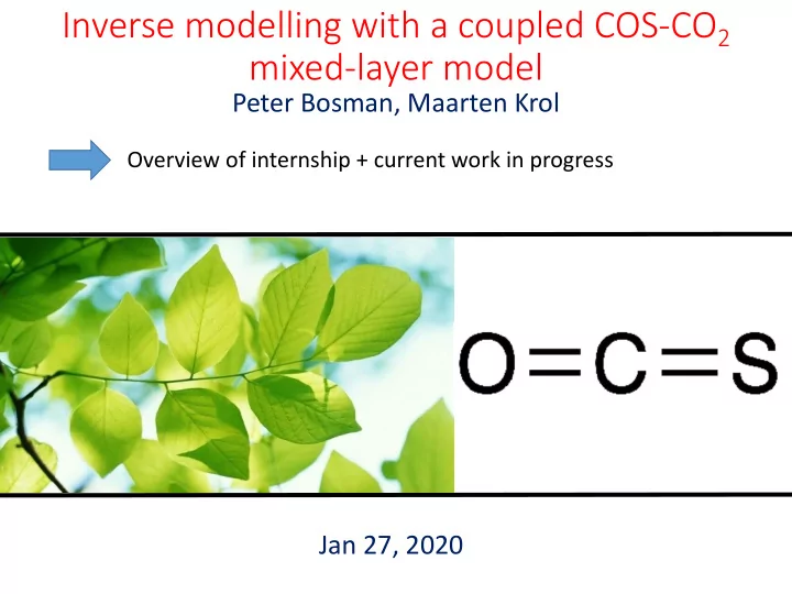
Inverse modelling with a coupled COS-CO 2 mixed-layer model Peter Bosman, Maarten Krol Overview of internship + current work in progress Jan 27, 2020

Vegetation uptake Largest COS sink CO2 CO2 CO2 Uptake by diffusion CO2 COS COS COS within leaves COS destroyed by CO2 CO2 enzymes COS Leaf stomata 2

COS uptake and photosynthesis coupled to stomatal conductance -> crucial link between COS and photosynthesis A-gs approach: Low for COS !"#$ = &'()#&*+(&, ∗ (&'(&,(*/+*0'( 0( +0/ − 0(*,/(+" &'(&,(*/+*0'() COS CO2 Stomatal + internal Canopy scale: integration over leaf area index CO 2 and COS often coupled via ratio of deposition velocities, in this study coupled via conductance 3

Inverse modelling vegetation fluxes with a coupled COS-CO 2 mixed-layer model Peter Bosman, Maarten Krol Overview of internship + current work in progress Jan 27, 2020

The model Height Mixed layer model CLASS Scalar (potential temperature, specific humidity, chemical species) 5

The model Free troposphere Entrainment Mixed layer Dynamic height Photosynthesis (A-g s ) Respiration COS exchange Surface heat fluxes Soil + vegetation Soil COS diffusion-reaction model implemented 6

This research Specific aim: Build an inverse modelling framework with a flexible cost function that allows for optimising different types of variables, including variables relating to the boundary layer dynamics simple approach! 7

The optimisation (max) 4 parameters optimised in this study: • alfa_plant à scaling conductance influences COS and CO 2 uptake Main link with boundary layer dynamics removed • alfa_soil à scaling soil COS uptake/emission influences COS uptake only • FTC_COS à free tropospheric concentration of COS • FTC_CO2_scale à scale for free tropospheric concentration of CO 2 8

Observations - Hyytiälä Dataset from boreal forest in Finland – Linda Kooijmans COS and CO 2 mixing ratios at 125 m eddy-covariance fluxes at 23 m +… Averaged over 7 sunny August days 9

Observations - Hyytiälä 10

Observations - Hyytiälä Cost function prior: 2067.45 Cost function optimised: 3.95 11

Observations - Hyytiälä Fluxes can be improved --> Add to cost function! 12

With net COS flux in cost function: 13

With net COS flux and gpp in cost function: 14

Challenges Derivative is approximated numerically (forward perturbation only) Analytical derivative requires construction of the adjoint model ≈ " # − " % Derivative at x A Δ' Cost function A B 15 Parameter x

Challenges Derivative is approximated numerically (forward perturbation only) Analytical derivative requires construction of the adjoint model Model is non-linear 16

Benefits of the framework Cost function can contain any variable with observations Any parameter can be optimised Future goal: No more messing with manual parameter fitting!! Challenges remain à Switch to analytical derivative? 17

Current work Free troposphere Entrainment: COS, CO 2 exchange Dynamic height Mixed layer Height Photosynthesis (A-gs) COS uptake by vegetation Surface layer CO 2 respiration Soil COS exchange Soil + vegetation Soil COS diffusion, [COS], [CO 2 ] production and destruction

Novelties and challenges In between ecosystem and global study Incorporate several type of obs Strongly nonlinear model Parameter dependency Cost function x 19 Prior

Current work Analytical derivative : construction of the mixed-layer adjoint 20

Adjoint modelling Model code: ! = 3 ∗ % + 5 ∗ ( Tangent linear model code: )! = 3 ∗ )% + 5 ∗ )( )! 0 5 3 )! = )( 0 1 0 )( )% 0 0 1 )% Transpose matrix: ,)! 0 0 0 ,)! = ,)( 5 1 0 ,)( 3 0 1 ,)% ,)% Adjoint model code: adA = 3 * adC + adA adB = 5 * adC + adB adC = 0

Adjoint model code example

Adjoint modelling

Extra slides 24

COS conductance issues Assume canopy consists of three leaves of same size, different stom resistance And C_air = 10 + + 5 10 4 ≠ 5 10 4 2 2 2 2 25 - -

Potential of the framework Free tropospheric concentration Free troposphere: Entrainment flux d [COS] $%" &'() = Mixed layer !" *+, ℎ%./ℎ" Plant COS flux Soil + vegetation Soil COS flux 26

Potential of the framework Free tropospheric concentration Free troposphere: Entrainment flux d [COS] $%" &'() = Mixed layer !" *+, ℎ%./ℎ" Plant COS flux Soil + vegetation Soil COS flux 27

COS conductance issues Assume canopy consists of three leaves of same size, different stom resistance And C_air = 10 ri: 2 2 2 rs: 3 8 2 rtot 5 10 4 Flux(= C_air/rtot) 2 1 2.5 Flux_avg 1.8333 Tot flux 3* 1.8333 rs_avg 4.3333 rtot_avg 6.3333 flux_avg 1.578947 Tot flux 3*1.578947 28

Parameters Harvard Harvard four parameters optimised, two fluxes in cost function alfa_plant alfa_soil FTC_COS (ppb) FTC_CO2_scale Prior 0.8 0.5 0.380 1 (364 ppm) Optimised 0.822 -4.674 0.361 1.063 (387 ppm) 29

Optimiser performance test Now three parameters alfa_plant alfa_soil FTC_COS Truth 1 1 0.37 ppb Prior 23 -1 0.3 ppb Optimised 30

Optimiser performance test Now three parameters alfa_plant alfa_soil FTC_COS Truth 1 1 0.37 ppb Prior 23 -1 0.3 ppb Optimised -1.10 -94.62 0.364 ppb 31

Current coupling COS-CO 2 33

Soil flux Hyytiala 34

Potential of the framework Free tropospheric concentration Free troposphere: Entrainment flux d [COS] $%" &'() = Mixed layer !" *+, ℎ%./ℎ" Plant COS flux Soil + vegetation CO 2 !! Soil COS flux 35

Vegetation uptake COS uptake and photosynthesis coupled to stomatal conductance -> crucial link between COS and photosynthesis Often a simple relation assumed: !ℎ#$#%&'$ℎ(%)% = +,- .!$/0( +, 4 123 +,- LRU = Leaf Relative Uptake COS in leaves destroyed by enzymes, with limited backward diffusion CO 2 in leaves often assimilated, but backward diffusion can be significant 36

37