Markov Random Fields: Inference and Estimation SPiNCOM reading - PowerPoint PPT Presentation
Markov Random Fields: Inference and Estimation SPiNCOM reading group April 24 th , 2017 Dimitris Berberidis Ack: Juan-Andres Bazerque 1 Probabilistic graphical models Set of random variables Graph represents joint Nodes
Markov Random Fields: Inference and Estimation SPiNCOM reading group April 24 th , 2017 Dimitris Berberidis Ack: Juan-Andres Bazerque 1
Probabilistic graphical models Set of random variables Graph represents joint Nodes correspond to random variables Edges imply relations between rv’s Some applications Speech recognition, computer vision Decoding Gene reg. networks, disease diagnosis Key idea: Graph models conditional independencies Two main tasks: Inference and Estimation Inference : Given observed , obtain (marginal) conditionals Estimation : Given samples estimate (and thus ) 2
Roadmap Bayesian networks basics Markov Random Fields Continuous valued MRFs Inference using Harmonic solution Structure estimation through l-1 penalized MLE Binary valued MRFs (Ising model) Inference Gaussian approximation – Random walk interpretation MCMC Structure estimation Pseudo MLE Logistic regression Conclusions 3
Directed Acyclical GMs (Bayesian networks) Ordered Markov property : Complete independence: Markov “Blanket” (Parents+children+co-parents) Joint pdf modeled as product of conditionals: Examples 2 nd order Markov chain Markov chain Naïve Bayes Hidden Markov model Arbitrary 4
Basic building blocks of Bayesian nets The chain structure The tent structure The V structure Berkson’s Paradox (“explaining away”) 5
Undirected GMs (Markov random fields) More natural in some domains (e.g. special statistics, relational data) Simple rule: Nodes not connected w. edge are conditionally independent Joint pdf parametrized and modeled as product of factors(not conditionals) Each factor or potential corresponds to a maximal clique Hamersley-Clifford theorem satisfies the CI properties of an undirected graph iff where Example Partition Function: Generally NP-hard to compute 6
Equivalence of DGMs and UGMs Moralization: Transition from directed to undirected GM Drop directionality and connect “unmarried’’ parents Information may be lost during transition (see example) lost due to this edge Cannot be represented Cannot be represented by DAGs by UGMs 7
MRFs with energy functions Clique potentials usually represented using an “energy” function Joint (Gibbs distribution) High probability states correspond to low energy configurations Any MRF can be decomposed to pairwise potentials (and energy functions) MRF is associative if measures difference btw and , and Gaussian MRF: Ising (binary +1,-1) model: 8
Gaussian MRFs Joint Gaussian fully parametrized by covariance and mean GMRF structure given by precision matrix (inv. Cov.) Also viewed as the Laplacian of the graph Assume for simplicity (and wlog) that Inference: Given known and observed , find 9
Inference via Harmonic solution Negative log-likelihood of joint Finally “Harmonic” Conditional mean of contains all information from observed 10
GMRF structure estimation via maximum likelihood Given , goal is to estimate and Log-likelihood 11
- penalized MLE of Closed-form solution: generally is full matrix Idea: Add constrain on to enforce (sparse) graph structure Problem is convex and for is equivalent to Solvable via Graphical Lasso O. Banerjee, L. El Ghaoui, and A. d'Aspremont, "Model selection through sparse maximum likelihood estimation for multivariate Gaussian or binary data," J. Machine Learning Research , vol. 9, pp. 485-516, June 2008. 12
Binary random variables Ising model Ising model for or Log partition function: Estimation: l-1 penalized maximum likelihood for Problem: combinatorialy complex to compute Two alternatives: is upper-bounded or avoided Similar problem for inference: can only be approximated 13
The role of in Ising model Claim: Proof: consider and Use the Ising model Plug in the expression above 14
Example: Image segmentation Use 2-D HMM (Ising as hidden layer) to infer “meaning’’ of image pixels Observed image Hidden layer: Pixel Class ( water, sky, etc ) 15
Inference via Gaussian field approximation Exact inference NP-hard Use surrogate continuous-values Gaussian random field: Compute exact Harmonic solution: Predictor of unknown labels via GMRF mean: Approximation of marginal posteriors: Random walk interpretation Imagine particle performing a random walk on (unobserved) graph Let normalized Laplacian be transition probability matrix Observed variables act as sink nodes where the walk ends Starting from node i, probability that walk ends in +1 node is 16
Inference via MCMC Collect samples from MC with as stationary distribution Gibbs sampler: One variable (node) sampled at every round t ( the rest are fixed ) Exploits (sparse) conditional dependence structure of MRF Observed nodes used as (fixed) boundary conditions Experiments indicate Gibbs smpl offers better inference in rect. Ising models More sophisticated MCMC methods achieve faster mixing (e.g. Wolfs algorithm) 17
Towards estimation: Bounding the partition function Goal: Find computable with polynomial complexity Consider partition such that Computing is still hard L. El Ghaoui, A. Gueye. “A Convex Upper Bound on the Log-Partition Function for Binary Graphical Models,” Journal of 18 Machine Learning Research , vol. 9, pp. 485–516, Mar. 2008.
Relaxation of the bound Relax Add redundant constrains Relax Upper-bound Claim: bound quality 19
Pseudo Maximum Likelihood Want to solve: Dual Substituting dual above 20
Logistic regression for Goal: Estimate while avoiding computation of Idea: consider node and its connections Separate Use as input and as output Logistic regression parametric estimation of Estimate as a byproduct Problem statement: re-write problem bellow for the Ising model P. Ravikumar, M. J. Wainwright and J. Lafferty. High-dimensional Ising model selection using -regularized logistic regression. To appear in the Annals of Statistics. Available at http://www.eecs.berkeley.edu 21
Estimation of We have: Taking the logarithm Substituting the log-likelihood Convex problem 22
Conclusions Graphical models Modeling pdfs using conditional dependencies Undirected models (MRFs) naturally modeled by graphs Inference in closed form for Gaussian MRFs Estimation of GMRFs as Laplacian fitting problem Inference and estimation approximations for binary MRFs (Ising model) Possible research directions Active sampling on binary MRFs using MCMC Active sampling for MRF structure estimation 23
Recommend
More recommend
Explore More Topics
Stay informed with curated content and fresh updates.
