Machine learning of a Higgs decay classifier via quantum annealing - PowerPoint PPT Presentation
Machine learning of a Higgs decay classifier via quantum annealing Presenter: Joshua Job 1 Reference: Solving a Higgs optimization problem with quantum annealing for machine learning, forthcoming, Nature Collaborators: Alex Mott 2 ,
Machine learning of a Higgs decay classifier via quantum annealing Presenter: Joshua Job 1 Reference: “Solving a Higgs optimization problem with quantum annealing for machine learning”, forthcoming, Nature Collaborators: Alex Mott 2 , Jean-Roch Vlimant 2 , Daniel Lidar 3 , Maria Spiropulu 2 Associations: 1. Department of Physics, Center for Quantum Information Science & Technology, University of Southern California 2. Department of Physics, California Institute of Technology 3. Departments of Electrical Engineering, Chemistry, and Physics, Center for Quantum Information Science & Technology, University of Southern California
The problem: Higgs detection at the Large ● Hadron Collider Quantum annealing overview ● ● Our technique: Quantum annealing for Outline machine learning ● Results Future directions ● ● Acknowledgements
The problem: Higgs detection at the Large Hadron Collider
The LHC: ● Large Hadron Collider -- 27km ring Cost: ~$4.5 billion ●
Basic challenge: ● LHC produces 600 million collisions/second, generating ~75TB/sec of data
Basic challenge: ● LHC produces 600 million collisions/second, generating ~75TB/sec of data Like the Biblical flood ●
Basic challenge: LHC produces 600 million ● collisions/second, generating ~75TB/sec of data Like the Biblical flood ● Cut down to something closer to ● Niagara Falls, 1GB/sec of data
What process are we looking for anyway? A Higgs decaying into two photons, i.e the H ⟶ γγ process Background processes are, for instance, gg ⟶ γγ events
How they do it: Nested sets of triggers ● selecting the most interesting events according to criteria determined by simulations, discarding ~99.999% of the events May depend in part on ● boosted decision trees (BDTs) and multilayer perceptrons (MLPs aka neural nets, DNNs)
How they do it: Once you have a set of ● interesting events, you still have to classify which are signal (real Higgs decays, <5% of remaining events) and which background (other Standard Model processes, >95% of remaining events) Again typically using ● MLPs/DNNs or BDTs
Challenges of BDTs/DNNs in this context: We don’t have any real ● signal and background events Training data is all from ● simulated data from event generators which, while generally accurate, can’t be fully trusted, and are more likely to be incorrect in the very high-level correlations BDTs and DNNs typically employ.
Challenges of BDTs/MLPs in this context: 2nd issue: ● interpretability MLPs are notoriously ● like black boxes, and while advances have been made in interpretation, still not easy to understand. BDTs are better but still nontrivial Would be better if we ● could directly interpret how it works and/or it gave us info about the important physics
Challenges of BDTs/MLPs in this context: Is there a potentially ● lighter, faster, more robust to simulation error, and/or more interpretable method we could use? Are there seemingly ● dead-end avenues that are opened up by newly developed special-purpose hardware, such as quantum annealers?
Our approach: QAML Quantum annealing for machine learning
Basic idea: boosting Idea: if each person has ● a (very) rough idea of what the correct answer is, then polling many people will give a pretty good guess Given a set of weak ● classifiers, each only slightly better than random guessing, you construct a strong classifier by combining their output
Weak classifiers In principle, can take any ● form, so long as it meets the aforementioned criteria What about our case? ● We’re going to build ● weak classifiers using a reduced representation of the distribution over kinematic variables. What are said variables? ●
Our basic kinematic variables
What do we want from our weak classifiers? Interpretable/informative Minimal sensitivity to errors in Fast to evaluate (we’re going to the event generators have many of them, so they can’t be slow)
What do we want from our weak classifiers? Interpretable/informative Minimal sensitivity to errors in Fast to evaluate (we’re going to the event generators have many of them, so they can’t Answer: Use only individual be slow) kinematic variables and their Answer: Ignore higher-order products/ratios, not higher-order correlations, only use functions Answer: Use a linear function of correlations of certain quantiles of the a few quantiles distribution, neglect tails
h(v) Math sketch: v +1 S is the signal distribution, B ● 1 background, v is the variable v low and v high are the 30th v shift ● v low/high and 70th percentiles of S , -1 b low and b high the percentiles v -1 on B at those values If b high < 0.7 then define v shift ● = v low -v , elseif b low > 0.7 then v shift = v-v high , else reject v ● Define v +1 and v -1 as the 10th and 90th percentile of the transformed S distribution With this formulation, the ● weak classifier is given by Do this for all the variables ● and products (or, if flipped flipped, the ratio)
Whither quantum annealing? ● So far, I haven’t so much as mentioned quantum mechanics We’re close though! ● ● The weights w haven’t been restricted so far ● Let’s choose to make them binary ○ Simpler optimization space as the weights are less sensitive to misspecification of h ○ Enables nice efficiency gains for optimization, ie W i = {0,1} conversion to a QUBO (quadratic, unconstrained binary optimization)
Constructing a QUBO problem Minimize:
What can you do with a QUBO? Run simulated annealing or Submit the problem to a parallel tempering algorithms quantum annealer to solve --- (fully classical) D-Wave QA processors solve QUBOs natively
Brief overview of quantum annealing
What is quantum Roughly, one initializes a system of two-state quantum systems (qubits), label the states {-1,+1} annealing? Initialize the system in a trivial Hamiltonian H(0) and allow it to find the ground state Slowly change the Hamiltonian, turning off H(0) and increasing the strength of target H P until H=H p This final Hamiltonian corresponds to your QUBO problem
What is quantum H(0) = annealing? H P = H P is effectively x has a ground state of proportional to |0 〉 + |1 〉 σ i H(0) has no interactions, so cools to ground state quickly, and the total ground state is an equal superposition over all bitstrings
Why quantum Because we can ● ● We suspect that with an appropriately designed quantum annealing? annealer one can find the ground state more quickly via tunneling than one can through simple thermalization alone Hardware and algorithms are developing rapidly, with ● feedback between producers (to date, primarily D-Wave Systems) and users, so we could effect the future trajectory of development
Our quantum Built by D-Wave ● Systems in Burnaby, annealer CA ● 1152 qubits nominal, 1098 functioning/active Chilled to 15mK ● Hardware graph: ● Red are inactive qubits ● Lines are couplers Green are active ● qubits
Our quantum Not fully connect ● ● But our problem is annealer minimizing That’s fully connected, the sum is over all i,j . What to do...
Minor embedding: Bind qubits in a chain together very tightly, When a chain with an energy that is J F times stronger than the feels like a qubit couplings of the problem Split local field across all qubits in the chain Decode states returned from the annealer by majority vote
Our problems: Training dataset is approximately 200k signal and ● background events (each), divided into 20 sets of 10k each to estimate random variation from dataset ● Testing set is approximately 100k events Signal data generated using 125 GeV Higgs decays ● produced by gluon fusion at 8TeV collisions using PYTHIA 6.4 ● Background data of Standard Model processes generated using SHERPA after restricting to processes that meet realistic trigger and detector acceptance requirements, p T 1 > 32 GeV, p T 2 > 25 GeV with diphoton mass 122.5 GeV < m γγ < 127.5 GeV and | η |<2.5 Used training sizes of 100, 1000, 5000, 10k, 15k, and ● 20k events, 20 such sets per size, and split evenly between signal and background
Our problems: Training dataset is approximately 200k signal and ● background events (each), divided into 20 sets of 10k each to estimate random variation from dataset ● Testing set is approximately 100k events Signal data generated using 125 GeV Higgs decays ● produced by gluon fusion at 8TeV collisions using PYTHIA 6.4 ● Background data of Standard Model processes generated using SHERPA after restricting to processes that meet realistic trigger and detector acceptance requirements, p T 1 > 32 GeV, p T 2 > 25 GeV with diphoton mass 122.5 GeV < m γγ < 127.5 GeV and | η |<2.5 Used training sizes of 100, 1000, 5000, 10k, 15k, and ● 20k events, 20 such sets per size, and split evenly between signal and background
Results, at long last
Recommend
More recommend
Explore More Topics
Stay informed with curated content and fresh updates.

