LQG for discrete-time systems Starting point and control strategy - PowerPoint PPT Presentation

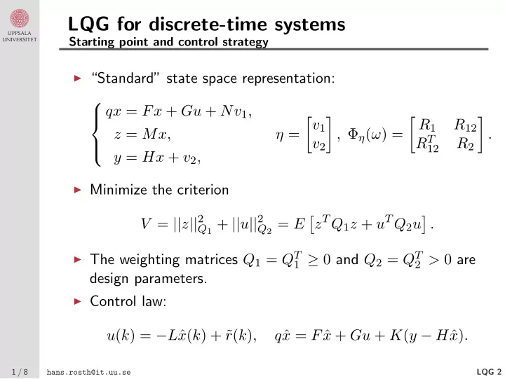
LQG for discrete-time systems Starting point and control strategy ◮ “Standard” state space representation:  qx = Fx + Gu + Nv 1 , � R 1  � v 1 � � R 12  z = Mx, η = , Φ η ( ω ) = . R T v 2 R 2 12  y = Hx + v 2 ,  ◮ Minimize the criterion z T Q 1 z + u T Q 2 u V = || z || 2 Q 1 + || u || 2 � � Q 2 = E . ◮ The weighting matrices Q 1 = Q T 1 ≥ 0 and Q 2 = Q T 2 > 0 are design parameters. ◮ Control law: u ( k ) = − L ˆ x ( k ) + ˜ r ( k ) , q ˆ x = F ˆ x + Gu + K ( y − H ˆ x ) . 1 / 8 hans.rosth@it.uu.se LQG 2

LQG: The optimal controller Theorem 9.4 ◮ The optimal control law is u ( k ) = − L ˆ x ( k | k − 1) , ◮ ˆ x ( k | k − 1) is obtained from the corresponding Kalman filter . ◮ The optimal state feedback gain is L = ( G T SG + Q 2 ) − 1 G T SF. ◮ The matrix S = S T ≥ 0 is the solution to the discrete-time Riccati equation (DARE) S = F T SF + M T Q 1 M − F T SG ( G T SG + Q 2 ) − 1 G T SF. ◮ N.B. There are two different DAREs involved, the one above and the one for the Kalman filter! ◮ Corollary 9.2: For the case when R 12 = 0 the control law u ( k ) = − L ˆ x ( k | k ) is the optimal controller with a direct/feed through term (so that u ( k ) depends on y ( k ) also). 2 / 8 hans.rosth@it.uu.se LQG 2

Example: Sampled LQ control of a DC motor The effect of Q 1 and Q 2 1 ◮ The DC-motor Y ( s ) = s ( s +1) U ( s ) , ◮ sampled with h = 0 . 1 ⇒ y ( k ) = 0 . 4837 · 10 − 2 ( q +0 . 9672) u ( k ) . ( q − 1)( q − 0 . 9048) ◮ u ( k ) = − Lx ( k ) + mr ( k ) , Q 1 = 1 = constant and Q 2 varied. 20 Q 2 = 10 −4 15 1 Q 2 = 0.01 10 0.8 5 Q 2 = 0.1 Q 2 = 1 0.6 y 0 u Q 2 = 0.1 Q 2 = 0.01 −5 Q 2 = 1 0.4 Q 2 = 10 −4 −10 0.2 −15 0 −20 0 1 2 3 4 5 6 0 0.5 1 1.5 2 time time ◮ Simulations: Step responses ( r = unit step) for the closed loop systems. The output y to the left, the input u to the right. 3 / 8 hans.rosth@it.uu.se LQG 2

Cross term in the criterion ◮ Sometimes there is a cross term in the criterion: z T Q 1 z + 2 x T Q 12 u + u T Q 2 u � � V = E ◮ Can be treated explicitely. ◮ Alternative: Bring it back to the standard case by a preliminary state feedback, u = u + Q − 1 2 Q T ˜ 12 x. ◮ This leads to the modified LQ-problem with Q 1 = M T Q 1 M − Q 12 Q − 1 ˜ ˜ ˜ 2 Q T M = I, 12 , Q 2 = Q 2 . ◮ The optimal control law is then u = − Lx = − ˜ Lx − Q − 1 2 Q T 12 x , i.e. L = ˜ L + Q − 1 2 Q T 12 . 4 / 8 hans.rosth@it.uu.se LQG 2

Continuous-time LQG by sampling controller Sampling the criterion function ◮ Continuous-time system ( A, B, M, C ). ◮ Sampling controller with sampling period h . ◮ Minimize the continuous-time criterion z T ( t ) Q 1 z ( t ) + u T ( t ) Q 2 u ( t ) � � V c = E . ◮ This is equivalent to minimizing the discrete-time criterion x T ( k ) ¯ Q 1 x ( k ) + 2 x T ( k ) ¯ Q 12 u ( k ) + u T ( k ) ¯ � � V d = E Q 2 u ( k ) , with � h 0 Ψ T Q 1 Ψ dt , ◮ ¯ Q 1 = � h 0 Γ T Q 1 Ψ dt , ◮ ¯ Q 12 = � h 0 Γ T Q 1 Γ dt + hQ 2 , ◮ ¯ Q 2 = � t where Ψ( t ) = Me At and Γ( t ) = 0 Ψ( s ) Bds . 5 / 8 hans.rosth@it.uu.se LQG 2

Example: The effect of the sampling period Intersample behaviour ◮ LQ control of the DC-motor. ◮ Two different sampling periods: h = 1 (left) and h = 0 . 1 (right). Output with cont.−time controller 1 1 0.8 0.8 Output for discr.−time systems y Outputs for discr.−time systems 0.6 y 0.6 Solid line: Sampling controller, discr.−time criterion Outputs for cont.− Dashed line: Sampling controller, sampled criterion −time systems with 0.4 cont.−time controller 0.4 and sampling Output for cont.−time systems controllers (coinciding) with sampling controllers 0.2 0.2 0 0 0 1 2 3 4 5 6 0 1 2 3 4 5 6 time time ◮ Identical weighting matrices, Q 1 = 1 and Q 2 = 0 . 01 , were used for ◮ continuous-time, ◮ discrete-time and ◮ sampled continuous-time versions of the criterion. 6 / 8 hans.rosth@it.uu.se LQG 2

LQG: Comments ◮ LQG optimal for given Q 1 and Q 2 , and under idealized conditions (exact model, R 1 and R 2 known etc) ◮ Q 1 and Q 2 are design parameters — use the optimization as a design tool, adjust Q 1 and Q 2 to get desirable properties for the closed loop system ◮ Q 1 penalizes z and Q 2 penalizes u , and only their relative sizes matter ◮ Q 1 and Q 2 usually diagonal matrices: if z i = [ z ] i is too big, increase the corresponding diagonal element q 1 i = [ Q 1 ] ii etc ◮ Too see any change of significance, Q 1 /Q 2 should be increased or decreased at least one order of magnitude (say 10 times) 7 / 8 hans.rosth@it.uu.se LQG 2

LQG: Comments, cont’d ◮ LQG gives an explicit solution for the optimization problem, and in the form of LTI filters F y ( q ) and F r ( q ) ( F y ( s ) and F r ( s ) in cont. time), which are easily implemented in a computer ◮ The design is an iterative process: check e.g. the sensitivity functions S and T , and simulate the closed loop system ◮ LQG requires a linear model, so limitations (e.g. bounds on u ) cannot be accounted for explicitely ◮ Useful Matlab functions: ◮ lqr, lqry, dlqr: compute L ◮ lqg, lqgreg: return the controller as LTI object ◮ lqrd: computes L for sampled cont.-time criterion 8 / 8 hans.rosth@it.uu.se LQG 2