Local, Unconstrained Function Optimization COMPSCI 527 Computer - - PowerPoint PPT Presentation

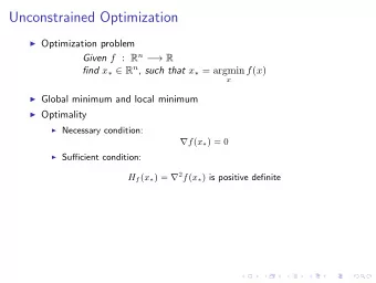
Local, Unconstrained Function Optimization

COMPSCI 527 — Computer Vision

Outline

1 Gradient, Hessian, and Convexity 2 A Local, Unconstrained Optimization Template 3 Steepest Descent 4 Termination 5 Convergence Speed of Steepest Descent 6 Convergence Speed of Newton’s Method 7 Newton’s Method 8 Counting Steps versus Clocking

Motivation and Scope

• Most estimation problems are solved by optimization
• Machine learning:
• Parametric predictor: h(x ; v) : Rd ⇥ Rm ! Y
• Risk: LT(v) = 1

N

PN

n=1 `(yn, h(xn ; v)) : Rm ! R

• Training:

ˆ v = arg minv2R

• 3D Reconstruction:

I = ⇡(C, S) where I are the images, C are the camera positions and orientations, S is scene shape

• Given I, find ˆ

C, ˆ S = arg minC,S kI ⇡(C, S)k

• In general, “solving” equation E(z) = 0 can be viewed as

ˆ z = arg minz kE(z)k

METERS

JAM

SCENE

C s

t

00

ft

EEhFE

T RAG T

Only Local Minimization

ˆ z = arg minz2? f(z)

• All we know about f is a “black box” (think Python function)
• For many problems, f has many local minima
• Start somewhere (z0), and take steps “down”

f(zk+1) < f(zk)

• When we get stuck at a local minimum, we declare success
• We would like global minima, but all we get is local ones
• For some problems, f has a unique minimum...
• ... or at least a single connected set of minima

2 C IRM

Gradient

rf(z) = ∂f

∂z =

2 6 4

∂f ∂z1

. . .

∂f ∂zm

3 7 5

• We saw the gradient for the case z 2 R2
• If rf(z) exists everywhere, the condition

rf(z) = 0 is necessary and sufficient for a stationary point (max, min, or saddle)

• Warning: only necessary for a minimum!
• Reduces to first derivative when f : R ! R

zEe

fC

g

k

q

2

forksomeday

First Order Taylor Expansion

f(z) ⇡ g1(z) = f(z0) + [rf(z0)]T(z z0) approximates f(z) near z0 with a (hyper)plane through z0

rf(z0) points to direction of steepest increase of f at z0

• If we want to find z1 where f(z1) < f(z0), going along

rf(z0) seems promising

• This is the general idea of steepest descent

ZER2

FE

Hessian

H(z) = 2 6 6 4

∂2f ∂z2

. . .

∂2f ∂z1∂zm

. . . . . .

∂2f ∂zm∂z1

. . .

∂2f ∂z2

3 7 7 5

• Symmetric matrix because of Schwarz’s theorem:

∂2f ∂zi∂zj = ∂2f ∂zj∂zi

• Eigenvalues are real because of symmetry
• Reduces to d2f

dz2 for f : R ! R

Convexity

• Convex everywhere:

For all z, z0 in the (open) domain of f and for all u 2 [0, 1] f(uz + (1 u)z0)  uf(z) + (1 u)f(z0)

• Convex at z0: The function f is convex everywhere in some
• pen neighborhood of z0

O

Convexity and Hessian

• If H(z) is defined at a stationary point z of f, then z is a

minimum iff H(z) < 0

• “<” means positive semidefinite:

zTHz 0 for all z 2 Rm

• Above is definition of H(z) < 0
• To check computationally: All eigenvalues are nonnegative
• H(z) < 0 reduces to d2f

dz2 0 for f : R ! R

Of E

Second Order Taylor Expansion

f ⇡ g2(z) = f(z0) + [rz0]T(z z0) + (z z0)TH(z0)(z z0) approximates f(z) near z0 with a quadratic equation through z0

• For minimization, this is useful only when H(z0) < 0
• Function looks locally like a bowl

• If we want to find z1 where f(z1) < f(z0), going to the

bottom of the bowl seems promising

• This is the general idea of Newton’s method

O

A Template

• Regardless of method, most local unconstrained
• ptimization methods fit the following template:

k = 0 while zk is not a minimum compute step direction pk with kpkk > 0 compute step size αk > 0 zk+1 = zk + αkpk k = k + 1 end.

GIVEN Eo

ITERATION COUNT

e

I

I

Design Decisions

• Whether to stop (“while zk is not a minimum”)
• In what direction to proceed (pk)
• How long a step to take in that direction (αk)
• Different decisions for the last two lead to different methods

with very different behaviors and computational costs