Clustering / Unsupervised Learning The target features are not given - PowerPoint PPT Presentation
Clustering / Unsupervised Learning The target features are not given in the training examples The aim is to construct a natural classification that can be used to predict features of the data. D. Poole and A. Mackworth 2019 c Artificial
Clustering / Unsupervised Learning The target features are not given in the training examples The aim is to construct a natural classification that can be used to predict features of the data. � D. Poole and A. Mackworth 2019 c Artificial Intelligence, Lecture 10.2 1 / 19
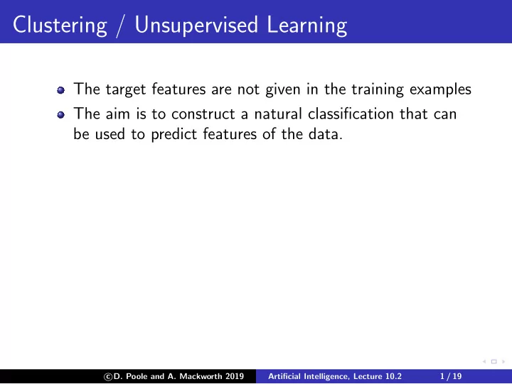
Clustering / Unsupervised Learning The target features are not given in the training examples The aim is to construct a natural classification that can be used to predict features of the data. The examples are partitioned in into clusters or classes. Each class predicts feature values for the examples in the class. ◮ In hard clustering each example is placed definitively in a class. ◮ In soft clustering each example has a probability distribution over its class. Each clustering has a prediction error on the examples. The best clustering is the one that minimizes the error. � D. Poole and A. Mackworth 2019 c Artificial Intelligence, Lecture 10.2 1 / 19
k -means algorithm The k -means algorithm is used for hard clustering. Inputs: training examples the number of classes, k Outputs: a prediction of a value for each feature for each class an assignment of examples to classes � D. Poole and A. Mackworth 2019 c Artificial Intelligence, Lecture 10.2 2 / 19
k -means algorithm formalized E is the set of all examples the input features are X 1 , . . . , X n X j ( e ) is the value of feature X j for example e . there is a class for each integer i ∈ { 1 , . . . , k } . � D. Poole and A. Mackworth 2019 c Artificial Intelligence, Lecture 10.2 3 / 19
k -means algorithm formalized E is the set of all examples the input features are X 1 , . . . , X n X j ( e ) is the value of feature X j for example e . there is a class for each integer i ∈ { 1 , . . . , k } . The k -means algorithm outputs function class : E → { 1 , . . . , k } . class ( e ) = i means e is in class i . prediction � X j ( i ) for each feature X j and class i . � D. Poole and A. Mackworth 2019 c Artificial Intelligence, Lecture 10.2 3 / 19
k -means algorithm formalized E is the set of all examples the input features are X 1 , . . . , X n X j ( e ) is the value of feature X j for example e . there is a class for each integer i ∈ { 1 , . . . , k } . The k -means algorithm outputs function class : E → { 1 , . . . , k } . class ( e ) = i means e is in class i . prediction � X j ( i ) for each feature X j and class i . The sum-of-squares error for class and � X j ( i ) is � D. Poole and A. Mackworth 2019 c Artificial Intelligence, Lecture 10.2 3 / 19
k -means algorithm formalized E is the set of all examples the input features are X 1 , . . . , X n X j ( e ) is the value of feature X j for example e . there is a class for each integer i ∈ { 1 , . . . , k } . The k -means algorithm outputs function class : E → { 1 , . . . , k } . class ( e ) = i means e is in class i . prediction � X j ( i ) for each feature X j and class i . The sum-of-squares error for class and � X j ( i ) is � � 2 n � � � X j ( class ( e )) − X j ( e ) . e ∈ E j =1 Aim: find class and prediction function that minimize sum-of-squares error. � D. Poole and A. Mackworth 2019 c Artificial Intelligence, Lecture 10.2 3 / 19
Minimizing the error The sum-of-squares error for class and � X j ( i ) is � � 2 � � n � X j ( class ( e )) − X j ( e ) . j =1 e ∈ E Given class , the � X j that minimizes the sum-of-squares error is � D. Poole and A. Mackworth 2019 c Artificial Intelligence, Lecture 10.2 4 / 19
Minimizing the error The sum-of-squares error for class and � X j ( i ) is � � 2 � � n � X j ( class ( e )) − X j ( e ) . j =1 e ∈ E Given class , the � X j that minimizes the sum-of-squares error is the mean value of X j for that class. � D. Poole and A. Mackworth 2019 c Artificial Intelligence, Lecture 10.2 4 / 19
Minimizing the error The sum-of-squares error for class and � X j ( i ) is � � 2 � � n � X j ( class ( e )) − X j ( e ) . j =1 e ∈ E Given class , the � X j that minimizes the sum-of-squares error is the mean value of X j for that class. Given � X j for each j , each example can be assigned to the class that � D. Poole and A. Mackworth 2019 c Artificial Intelligence, Lecture 10.2 4 / 19
Minimizing the error The sum-of-squares error for class and � X j ( i ) is � � 2 � � n � X j ( class ( e )) − X j ( e ) . j =1 e ∈ E Given class , the � X j that minimizes the sum-of-squares error is the mean value of X j for that class. Given � X j for each j , each example can be assigned to the class that minimizes the error for that example. � D. Poole and A. Mackworth 2019 c Artificial Intelligence, Lecture 10.2 4 / 19
k -means algorithm Initially, randomly assign the examples to the classes. Repeat the following two steps: For each class i and feature X j , � e : class ( e )= i X j ( e ) � X j ( i ) ← |{ e : class ( e ) = i }| , For each example e , assign e to the class i that minimizes � � 2 � n � X j ( i ) − X j ( e ) . j =1 until the second step does not change the assignment of any example. � D. Poole and A. Mackworth 2019 c Artificial Intelligence, Lecture 10.2 5 / 19
k -means algorithm Sufficient statistics: cc [ c ] is the number of examples in class c , fs [ j , c ] is the sum of the values for X j ( e ) for examples in class c . then define pn ( j , c ), current estimate of � X j ( c ) pn ( j , c ) = � D. Poole and A. Mackworth 2019 c Artificial Intelligence, Lecture 10.2 6 / 19
k -means algorithm Sufficient statistics: cc [ c ] is the number of examples in class c , fs [ j , c ] is the sum of the values for X j ( e ) for examples in class c . then define pn ( j , c ), current estimate of � X j ( c ) pn ( j , c ) = fs [ j , c ] / cc [ c ] � D. Poole and A. Mackworth 2019 c Artificial Intelligence, Lecture 10.2 6 / 19
k -means algorithm Sufficient statistics: cc [ c ] is the number of examples in class c , fs [ j , c ] is the sum of the values for X j ( e ) for examples in class c . then define pn ( j , c ), current estimate of � X j ( c ) pn ( j , c ) = fs [ j , c ] / cc [ c ] class ( e ) = � D. Poole and A. Mackworth 2019 c Artificial Intelligence, Lecture 10.2 6 / 19
k -means algorithm Sufficient statistics: cc [ c ] is the number of examples in class c , fs [ j , c ] is the sum of the values for X j ( e ) for examples in class c . then define pn ( j , c ), current estimate of � X j ( c ) pn ( j , c ) = fs [ j , c ] / cc [ c ] n � ( pn ( j , c ) − X j ( e )) 2 class ( e ) = arg min c j =1 These can be updated in one pass through the training data. � D. Poole and A. Mackworth 2019 c Artificial Intelligence, Lecture 10.2 6 / 19
1: procedure k-means ( Xs , Es , k ) Initialize fs and cc randomly (based on data) 2: def pn ( j , c ) = fs [ j , c ] / cc [ c ] 3: � n j =1 ( pn ( j , c ) − X j ( e )) 2 def class ( e ) = arg min c 4: repeat 5: fsn and ccn initialized to be all zero 6: for each example e ∈ Es do 7: c := class ( e ) 8: ccn [ c ]+ = 1 9: for each feature X j ∈ Xs do 10: fsn [ j , c ]+ = X j ( e ) 11: stable := ( fsn = fs ) and ( ccn = cc ) 12: fs := fsn 13: cc := ccn 14: until stable 15: return class , pn 16: � D. Poole and A. Mackworth 2019 c Artificial Intelligence, Lecture 10.2 7 / 19
Example Data 10 8 6 4 2 0 0 2 4 6 8 10 � D. Poole and A. Mackworth 2019 c Artificial Intelligence, Lecture 10.2 8 / 19
Random Assignment to Classes 10 8 6 4 2 0 0 2 4 6 8 10 � D. Poole and A. Mackworth 2019 c Artificial Intelligence, Lecture 10.2 9 / 19
Assign Each Example to Closest Mean 10 8 6 4 2 0 0 2 4 6 8 10 � D. Poole and A. Mackworth 2019 c Artificial Intelligence, Lecture 10.2 10 / 19
Ressign Each Example to Closest Mean 10 8 6 4 2 0 0 2 4 6 8 10 � D. Poole and A. Mackworth 2019 c Artificial Intelligence, Lecture 10.2 11 / 19
Properties of k -means An assignment of examples to classes is stable if running both the M step and the E step does not change the assignment. This algorithm will eventually converge to a stable local minimum. Any permutation of the labels of a stable assignment is also a stable assignment. It is not guaranteed to converge to a global minimum. It is sensitive to the relative scale of the dimensions. Increasing k can always decrease error until k is the number of different examples. � D. Poole and A. Mackworth 2019 c Artificial Intelligence, Lecture 10.2 12 / 19
EM Algorithm Used for soft clustering — examples are probabilistically in classes. k -valued random variable C Model Data Probabilities ➪ X 1 X 2 X 3 X 4 P ( C ) t f t t P ( X 1 | C ) C f t t f P ( X 2 | C ) f f t t P ( X 3 | C ) X 1 X 2 X 3 X 4 · · · P ( X 4 | C ) � D. Poole and A. Mackworth 2019 c Artificial Intelligence, Lecture 10.2 13 / 19
EM Algorithm M-step X 1 X 2 X 3 X 4 C count . . . . . . P ( C ) . . . . . . . . . . . . P ( X 1 | C ) t f t t 1 0.4 P ( X 2 | C ) t f t t 2 0.1 P ( X 3 | C ) t f t t 3 0.5 P ( X 4 | C ) . . . . . . . . . . . . . . . . . . E-step � D. Poole and A. Mackworth 2019 c Artificial Intelligence, Lecture 10.2 14 / 19
Recommend
More recommend
Explore More Topics
Stay informed with curated content and fresh updates.
