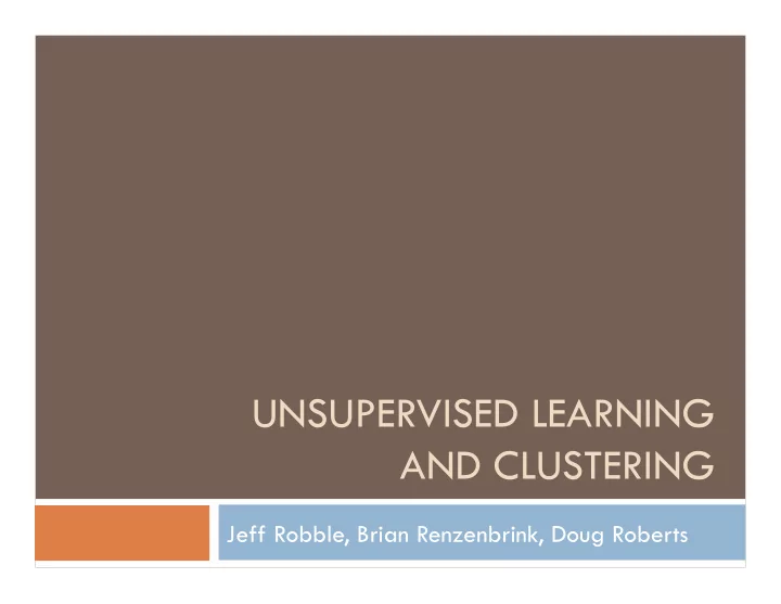
UNSUPERVISED LEARNING AND CLUSTERING Jeff Robble, Brian - PowerPoint PPT Presentation

UNSUPERVISED LEARNING AND CLUSTERING Jeff Robble, Brian Renzenbrink, Doug Roberts

Unsupervised Procedures A procedure that uses unlabeled data in its classification process. Why would we use these?  Collecting and labeling large data sets can be costly  Occasionally, users wish to group data first and label the groupings second  In some applications, the pattern characteristics can change over time. Unsupervised procedures can handle these situations.  Unsupervised procedures can be used to find useful features for classification  In some situations, unsupervised learning can provide insight into the structure of the data that helps in designing a classifier

Unsupervised vs. Supervised Unsupervised learning can be thought of as finding patterns in the data above and beyond what would be considered pure unstructured noise. How does it compare to supervised learning? With unsupervised learning it is possible to learn larger and more complex models than with supervised learning. This is because in supervised learning one is trying to find the connection between two sets of observations, while unsupervised learning tries to identify certain latent variables that caused a single set of observations. The difference between supervised learning and unsupervised learning can be thought of as the difference between discriminant analysis from cluster analysis.

Mixture Densities We assume that p( x | ω j ) can be represented in a functional form that is determined by the value of parameter vector θ j . For example, if we have p( x | ω j ) ~ N( µ j , Σ j ), where N is the function for a normal gaussian distribution and θ j consists of the components µ j and Σ j that characterize the average and variance of the distribution. We need to find the probability of x for a given ω j and θ , but we don’t know the exact values of the θ components that go into making the decision. We need to solve: P ( ω j | x ) = p ( x | ω j ) P ( ω j ) p ( x ) but instead of p( x | ω j ) we have p( x | ω j , θ j ). We can solve for the mixture density: c ∑ p ( x | θ ) = p ( x | ω j , θ j ) P ( ω j ) (1) j = 1

Mixture Densities c ∑ p ( x | θ ) = p ( x | ω j , θ j ) P ( ω j ) (1) j = 1 component densities mixing parameters We make the following assumptions:  The samples come from a known number of c classes.  The prior probabilities P( ω j ) for each class are known, j = 1…c.  The forms for the class-conditional probability densities p( x | ω j , θ j ) are known, j = 1…c.  The values for the c parameter vectors θ 1 ... θ c are unknown.  The category labels are unknown  unsupervised learning. Consider the following mixture density where x is binary: P ( x | θ ) = 1 x (1 − θ 1 ) 1 − x + 1 x (1 − θ 2 ) 1 − x 2 θ 1 2 θ 2

Identifiability: Estimate Unknown Parameter Vector θ  1 2 ( θ 1 + θ 2 ) if x =1  P ( x | θ ) = 1 x (1 − θ 1 ) 1 − x + 1 x (1 − θ 2 ) 1 − x = 2 θ 1 2 θ 2  1 − 1  2 ( θ 1 + θ 2 ) if x = 0  Suppose we had an unlimited number of samples and use nonparametric methods to determine p(x| θ ) such that P(x=1| θ )=.6 and P(x=0| θ )=.4: Try to solve for θ 1 and θ 2 : 1 We discover that the mixture distribution is 2 ( θ 1 + θ 2 ) = .6 completely unidentifiable. We cannot infer the   − 1 − 1 individual parameters of θ . 2 ( θ 1 + θ 2 ) = .4     A mixture density, p( x | θ ) is identifiable if we can -1+ θ 1 + θ 2 = .2 recover a unique θ such that p( x | θ ) ≠ p( x | θ ’ ). θ 1 + θ 2 = 1.2

Maximum Likelihood Estimates The posterior probability becomes: P ( ω i | x k , θ ) = p ( x k | ω i , θ i ) P ( ω i ) (6) p ( x k | θ ) We make the following assumptions:  The elements of θ i and θ j are functionally independent if i ≠ j.  p(D| θ ) is a differentiable function of θ , where D = { x 1 , … , x n } of n independently drawn unlabeled samples. The search for a maximum value of p(D| θ ) extending over θ and P( ω j ) is constrained so that: c ∑ P ( ω i ) ≥ 0 i = 1,..., c and P ( ω i ) = 1 i=1 Let ˆ ( ω i ) be the maximim likelihood estimate for P ( ω i ). P Let ˆ i be the maximim likelihood estimate for θ i . θ ( ω i ) = 1 n ( ω i | x k , ˆ If ˆ ( ω i ) ≠ 0 for any i then ˆ ˆ ∑ P P P ) θ (11) n k = 1

Maximum Likelihood Estimates ( ω i ) = 1 n ( ω i | x k , ˆ ˆ ˆ ∑ P P ) θ (11) n k = 1 The MLE of the probability of a category is the average over the entire data set of the estimate derived from each sample (weighted equally) p ( x k | ω i ,ˆ i ) ˆ P ( ω i ) θ ( ω i | x k , ˆ ˆ P ) = θ (13) c p ( x k | ω j ,ˆ θ j ) ˆ ∑ P ( ω j ) j = 1 Bayes theorem. When estimating the probability for ω i , the numerator depends on ˆ i and not on the full ˆ . θ θ

Maximum Likelihood Estimates The gradient must vanish at the value of θ i that maximizes the logarithm of the likelihood, so the MLE ˆ i must satsify the following conditions: θ n ( ω i | x k , ˆ ∇ θ i ln p ( x k | ω i ,ˆ ˆ ∑ P ) i ) = 0 i =1,...,c θ θ (12) k = 1 Consider one sample, so n =1. Since we assumed ˆ P ≠ 0, the probability is maximized as a function of θ i so ∇ θ i ln p ( x k | ω i ,ˆ i ) = 0. Note that θ ln(1) = 0, so we are trying to find the a value of ˆ i that maximizes p(.). θ

Applying MLE to Normal Mixtures Case 1 : The only unknown quantities are the mean vectors . consists of components of The likelihood of this particular sample is and its derivative is Thus, according to Equation 8 in the book the MLE estimate must satisfy: where

Applying MLE to Normal Mixtures If we multiply the above equation by the covariance matrix and rearranging terms, we obtain the equation for the maximum likelihood estimate of the mean vector However, we still need to calculate explicitly. If we have a good initial estimate we can use a hill climbing procedure to improve our estimates

Applying MLE to Normal Mixtures Case 2: The mean vector , the covariance matrix , and the prior probabilities are all unknown In this case the maximum likelihood principle only gives singular solutions. Usually, singular solutions are unusable. However, if we restrict our attention to the largest of the finite local maxima of the likelihood function we can still find meaningful results. Using , , and derived from Equations 11-13 we can find the likelihood of using

Applying MLE to Normal Mixtures The differentiation of the previous equation gives and Where is the Kronecker delta, is the p th element of , is the p th element of , and is the pq th element of and

Applying MLE to Normal Mixtures Using the above differentiation along with Equation 12 we can find the following equations for the MLE of , , and

Applying MLE to Normal Mixtures These equations work where p ( x k | ω i , ˆ i ) ˆ P ( ω i ) θ ( ω i | x k , ˆ ˆ P θ ) = c p ( x k | ω j , ˆ ) ˆ ∑ P ( ω j ) θ j = 1 To solve the equation for the MLE, we should again start with an initial estimate to evaluate Equation 27, and use Equations 24-26 to update these estimates.

k-Means Clustering Clusters numerical data in which each cluster has a center called the mean The number of clusters c is assumed to be fixed The goal of the algorithm is to find the c mean vectors µ 1 , µ 2 , …, µ c The number of clusters c • May be guessed • Assigned based on the final application

k-Means Clustering The following pseudo code shows the basic functionality of the k -Means algorithm begin initialize n, c, µ 1 , µ 2 , …, µ c do classify n samples according to nearest µ i recompute µ i until no change in µ i return µ 1 , µ 2 , …, µ c end

k-Means Clustering Two dimensional example with c = 3 clusters Shows the initial cluster centers and their associated Voronoi tesselation Each of the three Voronoi cells are used to calculate new cluster centers

Fuzzy k-Means The algorithm assumes that each sample x j has a fuzzy membership in a cluster(s) The algorithm seeks a minimum of a heuristic global cost function Where:  b is a free parameter chosen to adjust the “blending” of clusters  b > 1 allows each pattern to belong to multiple clusters (fuzziness)

Fuzzy k-Means Probabilities of cluster membership for each point are normalized as Cluster centers are calculated using Eq. 32 Where:

Fuzzy k-Means The following is the pseudo code for the Fuzzy k-Means algorithm begin initialize n, c, b, µ 1 , …, µ c , , i = 1,…,c; j = 1,…,n normalize by Eq. 30 do recompute µ i by Eq. 32 recompute by Eq. 33 until small change in µ i and return µ 1 , µ 2 , …, µ c end

Fuzzy k-means Illustrates the progress of the algorithm Means lie near the center during the first iteration since each point has non-negligible “membership” Points near the cluster boundaries can Have membership in more that one cluster

x-Means In k-Means the number of clusters is chosen before the algorithm is applied In x-Means the Bayesian information criterion (BIC) is used globally and locally to find the best number of clusters k BIC is used globally to choose the best model it encounters and locally to guide all centroid splits