Unconstrained Optimization Optimization problem Given f : R n R - PowerPoint PPT Presentation

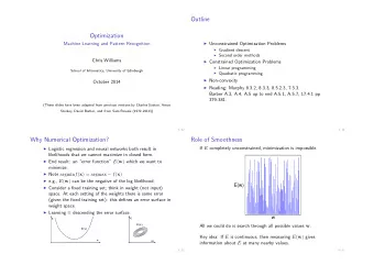
Unconstrained Optimization ◮ Optimization problem Given f : R n − → R find x ∗ ∈ R n , such that x ∗ = argmin f ( x ) x ◮ Global minimum and local minimum ◮ Optimality ◮ Necessary condition: ∇ f ( x ∗ ) = 0 ◮ Sufficient condition: H f ( x ∗ ) = ∇ 2 f ( x ∗ ) is positive definite

Newton’s method ◮ Taylor series approximation of f at k -th iterate x k : f ( x ) ≈ f ( x k ) + ∇ f ( x k ) T ( x − x k ) + 1 2( x − x k ) T H f ( x k )( x − x k ) ◮ Differentiating with respect to x and setting the result equal to zero yields the ( k + 1) -th iterate, namely Newton’s method : x k +1 = x k − [ H f ( x k )] − 1 ∇ f ( x k ) . ◮ Newton’s method converges quadratically when x 0 is near a minimum.

Gradient descent optimization ◮ Directional derivative of f at x in the direction u : 1 h [ f ( x + hu ) − f ( x )] = u T ∇ f ( x ) . D u f ( x ) = lim h → 0 D u f ( x ) measures the change in the value of f relative to the change in the variable in the direction of u . ◮ To min f ( x ) , we would like to find the direction u in which f decreases the fastest. ◮ Using the directional derivative, u u T ∇ f ( x ) = min min u � u � 2 �∇ f ( x ) � 2 cos θ = −�∇ f ( x ) � 2 2 when u = −∇ f ( x ) . ◮ u = −∇ f ( x ) is call the steepest descent direction.

Gradient descent optimization ◮ The steepest descent algorithm: x k +1 = x k − τ · ∇ f ( x k ) , where τ is called stepsize or “ learning rate ” ◮ How to pick τ ? 1. τ = argmin α f ( x k − α · ∇ f ( x k )) (line search) 2. τ = small constant 3. evaluate f ( x − τ ∇ f ( x )) for several different values of τ and choose the one that results in the smallest objective function value.

Example: solving the least squares by gradient-descent ◮ Let A ∈ R m × n and b = ( b i ) ∈ R m ◮ The least squares problem, also known as linear regression: 1 2 � Ax − b � 2 min x f ( x ) = min 2 x m 1 � f 2 = min i ( x ) 2 x i =1 where f i ( x ) = A ( i, :) T x − b i ◮ Gradient: ∇ f ( x ) = A T Ax − A T b ◮ The method of gradient descent: ◮ set the stepsize τ and tolerance δ to small positive numbers. ◮ while � A T Ax − A T b � 2 > δ do x ← x − τ · ( A T Ax − A T b )

Solving LS by gradient-descent MATLAB demo code: lsbygd.m ... r = A’*(A*x - b); xp = x - tau*r; res(k) = norm(r); if res(k) <= tol, ... end ... x = xp; ...

Connection with root finding Solving nonlinear system of equations: f 1 ( x 1 , x 2 , . . . , x n ) = 0 f 2 ( x 1 , x 2 , . . . , x n ) = 0 . . . f n ( x 1 , x 2 , . . . , x n ) = 0 is equivalent to solve the optimization problem n � ( f i ( x 1 , x 2 , . . . , x n )) 2 min x g ( x ) = g ( x 1 , x 2 , . . . , x n ) = i =1