Local Distributed Sampling ! om Locally - Defined Distribution - PowerPoint PPT Presentation
Local Distributed Sampling ! om Locally - Defined Distribution Yitong Yin Nanjing University Counting and Sampling [Jerrum-Valiant-Vazirani 86]: (For self-reducible problems) approx. counting (approx., exact) sampling is tractable is
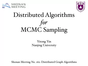
Local Distributed Sampling ! om Locally - Defined Distribution Yitong Yin Nanjing University
Counting and Sampling [Jerrum-Valiant-Vazirani ’86]: (For self-reducible problems) approx. counting (approx., exact) sampling is tractable is tractable
Computational Phase Transition Sampling almost-uniform independent set in graphs with maximum degree ∆ : • [Weitz 2006] : If ∆≤ 5 , poly-time. • [Sly 2010] : If ∆≥ 6 , no poly-time algorithm unless NP = RP . A phase transition occurs when ∆ : 5 → 6 . Local Computation?
Local Computation “ What can be computed locally? ” [Naor, Stockmeyer ’93] the LOCAL model [Linial ’87] : • Communications are synchronized. • In each round: each node can exchange unbounded messages with all neighbors, perform unbounded local computation, and read/write to unbounded local memory. • Complexity: # of rounds to terminate in the worst case. • In t rounds: each node can collect information up to distance t . PLOCAL: t = polylog( n )
A Motivation: Distributed Machine Learning • Data are stored in a distributed system. • Distributed algorithms for: • sampling from a joint distribution (specified by a probabilistic graphical model ); • inferring according to a probabilistic graphical model.
Example : Sample Independent Set µ : uniform distribution of independent sets in G . Y ∈ {0,1} V indicates an independent set • Each v ∈ V returns a Y v ∈ {0,1} , such that Y = ( Y v ) v ∈ V ∼ µ • Or: d TV ( Y , µ ) < 1/poly( n ) network G ( V , E )
Inference (Local Counting) µ : uniform distribution of independent sets in G . : marginal distribution at v conditioning on σ ∈ {0,1} S . µ σ v ∀ y ∈ { 0 , 1 } : v ( y ) = Pr Y ∼ µ [ Y v = y | Y S = σ ] µ σ 0 • Each v ∈ S receives σ v as input. • Each v ∈ V returns a marginal 0 distribution such that: µ σ ˆ v 1 1 1 d TV (ˆ v ) ≤ µ σ v , µ σ poly( n ) n 1 Y Z = µ ( ∅ ) = Y ∼ µ [ Y v i = 0 | ∀ j < i : Y v j = 0] Pr network G ( V , E ) i =1 Z : # of independent sets
Decay of Correlation : marginal distribution at v conditioning on σ ∈ {0,1} S . µ σ v strong spatial mixing (SSM): ∀ boundary condition B ∈ {0,1} r -sphere( v ) : v , µ σ ,B d TV ( µ σ ) ≤ poly( n ) · exp( − Ω ( r )) v SSM (iff ∆≤ 5 when µ is uniform G distribution of ind. sets) r approx. inference is solvable v B in O(log n ) rounds σ in the LOCAL model
Gibbs Distribution (with pairwise interactions) • Each vertex corresponds to a network G ( V , E ): variable with finite domain [ q ] . • Each edge e =( u , v ) ∈ E has a matrix (binary constraint): A e v u b v A e : [ q ] × [ q ] → [0,1] • Each vertex v ∈ V has a vector (unary constraint): b v : [ q ] → [0,1] • Gibbs distribution µ : ∀ σ ∈ [ q ] V Y Y µ ( σ ) ∝ A e ( σ u , σ v ) b v ( σ v ) e =( u,v ) ∈ E v ∈ V
Gibbs Distribution (with pairwise interactions) • Gibbs distribution µ : ∀ σ ∈ [ q ] V network G ( V , E ): Y Y µ ( σ ) ∝ A e ( σ u , σ v ) b v ( σ v ) e =( u,v ) ∈ E v ∈ V • independent set: A e v u b v 1 � 1 � 1 A e = b v = 1 0 1 • coloring: 0 1 1 A e : [ q ] × [ q ] → [0,1] 0 . . b v = A e = ... . 1 b v : [ q ] → [0,1] 1 0
Gibbs Distribution • Gibbs distribution µ : ∀ σ ∈ [ q ] V network G ( V , E ): Y µ ( σ ) ∝ f ( σ S ) ( f,S ) ∈ F each ( f, S ) ∈ F S is a local constraints (factors): f : [ q ] S → R ≥ 0 S ⊆ V with diam G ( S ) = O (1)
Locality of Counting & Sampling For Gibbs distributions (defined by local factors): Inference: Sampling: Correlation Decay: local approx. local approx. SSM inference sampling easy with additive error O(log 2 n ) factor local approx. local exact inference sampling with multiplicative error distributed Las Vegas sampler
Locality of Sampling Inference: Sampling: Correlation Decay: local approx. local approx. SSM inference sampling return a random Y = ( Y v ) v ∈ V each v can compute a µ σ ˆ v within O(log n ) -ball whose distribution ˆ µ ≈ µ 1 s.t. 1 d TV (ˆ µ, µ ) ≤ d TV (ˆ v ) ≤ µ σ v , µ σ poly( n ) poly( n ) sequential O(log n ) -local procedure: • scan vertices in V in an arbitrary order v 1 , v 2 , …, v n • for i =1,2, …, n : sample according to Y v 1 ,...,Y vi − 1 Y v i ˆ µ v i
Network Decomposition C colors ( C , D ) -network-decomposition of G : • classifies vertices into clusters; • assign each cluster a color in [ C ] ; • each cluster has diameter ≤ D ; r • clusters are properly colored. rD ( C , D ) r -ND: ( C , D ) -ND of G r Given a ( C , D ) r - ND: sequential r -local procedure: r = O(log n ) r = O(log n ) • scan vertices in V in an arbitrary order v 1 , v 2 , …, v n • for i =1,2, …, n : sample according to Y v 1 ,...,Y vi − 1 Y v i ˆ µ v i can be simulated in O( CDr ) rounds in LOCAL model
Network Decomposition O(log n ) colors ( C , D ) -network-decomposition of G : • classifies vertices into clusters; • assign each cluster a color in [ C ] ; • each cluster has diameter ≤ D ; O(log n ) • clusters are properly colored. O(log 2 n ) ( C , D ) r -ND: ( C , D ) -ND of G r ( O(log n ), O(log n )) r -ND can be constructed in O( r log 2 n ) rounds w.h.p. [Linial, Saks, 1993] — [Ghaffari, Kuhn, Maus, 2017]: r -local SLOCAL algorithm: O( r log 2 n ) -round LOCAL alg.: ND ∀ ordering π =( v 1 , v 2 , …, v n ) , returns w.h.p. the Y ( π ) for some ordering π returns random vector Y ( π )
Locality of Sampling Inference: Sampling: Correlation Decay: O(log n )- round O(log 3 n )- round local approx. local approx. SSM inference sampling with additive error local approx. local exact inference sampling with multiplicative error distributed Las Vegas sampler
An LLL -like Framework independent random variables: X 1 , …, X n with domain Ω A : a set of bad events variable set ( vbl ( A ) ⊆ [ n ] each is associated with A ∈ A { } q A : Ω vbl ( A ) → [0 , 1] function variable-framework Lovász local lemma Rejection sampling: ( with conditionally mutually independent filters ) • X 1 , …, X n are drawn independently; • each occurs independently with prob. ; � � A ∈ A 1 − q A X vbl ( A ) • the sample is accepted if none of occurs. A ∈ A Target distribution D * : X 1 , …, X n conditioned on accepted Partial rejection sampling [Guo-Jerrum-Liu’17] : resample not all variables Resample variables local to the errors? (Moser-Tardos)
Local Rejection Sampling • draw independent samples of X = ( X 1 , …, X n ) ; • each occurs ( violated ) ind. with Pr[ A ]=1- q A ( X vbl ( A ) ) ; A ∈ A • while there is a violated bad event : X old ← current X A ∈ A • resample all variables in vbl ( A ) for violated A ; • for violated A : violate A with Pr[ A ] = 1- q A ( X vbl ( A ) ) ; • for non-violated A that shares variables with violated event: ⇣ ⌘ violate A with Pr[ A ] = � � X old 1 − q ∗ A · q A X vbl ( A ) /q A vbl ( A ) where q A* is a worst-case lower bound for q A ( ) : � � ≥ q ∗ ∀ X vbl ( A ) : q A X vbl ( A ) A (target soft filters: ∀ A ∈ A , q ∗ ( X 1 , …, X n ) ~ D * A > 0 distribution) upon termination Only the variables local to the violated events are resampled. (work even for dynamic filters) By a resampling table argument.
Local Ising Sampler 0 < β < 1 external λ � β � 1 � 1 β ferro: anti-ferro: A = b = A = field β 1 λ > 0 β 1 1 • each vertex v ∈ V ind. samples a spin state σ v ∈ {0,1} ∝ b ; • each edge e =( u , v ) ∈ E fails ind. with prob. 1- A ( σ u , σ v ) ; • while there is a failed edge: σ old ← current σ • resample σ v for all vertices v involved in failed edges; • each failed e =( u , v ) is revived ind. with prob. A ( σ u , σ v ) ; • each non-failed e =( u , v ) that is incident to a failed edge, fails ind. with prob. 1 - β · A ( σ u , σ v )/ A ( σ u old , σ v old ) ; Cons : Pros : • convergence is hard to • local & parallel • dynamic graph analyze • regime is not tight • exact sampler β > 1 − Θ ( 1 ∆ ) • soft constraints • certifiable termination
Locality of Sampling For Gibbs distributions (distributions defined by local factors): Inference: Sampling: Correlation Decay: local approx. local approx. SSM inference sampling with additive error local approx. local exact inference sampling with multiplicative error distributed Las Vegas sampler
Jerrum-Valiant-Vazirani Sampler [ J errum- V aliant- V azirani ’86] ∃ an efficient algorithm that samples from ˆ µ µ ( σ ) given any σ ∈ { 0 , 1 } V and evaluates ˆ e − 1 /n 2 ≤ ˆ µ ( σ ) multiplicative error: ∀ σ ∈ { 0 , 1 } V : µ ( σ ) ≤ e 1 /n 2 Self-reduction: n n Z ( σ 1 , . . . , σ i ) Y µ σ 1 ,..., σ i − 1 Y µ ( σ ) = ( σ i ) = v i Z ( σ 1 , . . . , σ i − 1 ) i =1 i =1 ˆ Z ( σ 1 , . . . , σ i ) let Z ( σ 1 , . . . , σ i − 1 ) ≈ e ± 1 /n 3 · µ σ 1 ,..., σ i − 1 µ σ 1 ,..., σ i − 1 ˆ ( σ i ) = ( σ i ) v i v i ˆ e − 1 / 2 n 3 ≤ ˆ where by approx. counting Z ( ··· ) Z ( ··· ) ≤ e 1 / 2 n 3
Recommend
More recommend
Explore More Topics
Stay informed with curated content and fresh updates.
