Linear Transformation Transformation Linear with CG & - PDF document
Linear Transformation Transformation Linear with CG & animation with CG & animation Ogose Shigeki Ogose Shigeki Kawai- -Juku Juku Kawai Tokyo, Japan Tokyo, Japan http://mixedmoss.com/atcm/2012/
Linear Transformation Transformation Linear with CG & animation with CG & animation Ogose Shigeki Ogose Shigeki Kawai- -Juku Juku Kawai Tokyo, Japan Tokyo, Japan http://mixedmoss.com/atcm/2012/ http://mixedmoss.com/atcm/2012/ 1. Advantages of using Computer Graphics (CG). • Grids can be drawn easily. • Effects of changing the ‘ original objects ’ or ‘ matrix ’ can be seen immediately. • Exotic objects such as photos can be transformed. • Animations can be used.
Example of linear i ty − 2 1 ��� � ��� � ���� � ���� � ex 1. Transformatio n by 1 + → + 2 OA 3OB 2 OA' 3O B' 1 muffine.jar (0,1) (-1,1) (2,1) (1,0) original transformed θ − θ cos sin θ = ex2 . Transformation of a photo b y R ( ) θ θ sin c o s muffine.jar Use a palette or type it in the field. ° ° ( cos30 ,sin 30 ) − ° ° ( sin30 c , os30 ) original transformed
− 2 1 = ex3. Animation of Rotation&Enlargement by F 1 2 animation by rotation current matrix is 1 0 0 1 current matrix is − 2 1 1 2 Curr ent matrix is right-at-the-moment matrix. Which starts from the unit matrix and finishes as the target matrix. 2. EigenVectors & Animation Animation is useful for rotation - which has no real eigenvectors- , but it works even better for transformations which have real eigenvectors. Next example has 2 eigenvectors.
ex4. Comparison of 2 transformations which have same eigenvalues. 5 0 1 1 A 0 0 = = = For A A 5 , 2 , 0 2 0 0 1 1 1 0 eigenvectors : & , eigenvalues :5&2 , respectively. 0 1 − − 3 2 1 1 2 2 = = = For B , B 5 · , B 2 · 1 4 1 1 1 1 − 1 2 eigenvectors : & , eigenvalues :5&2 , respectively. 1 1 5 0 1 0 = Transformation by A . When the base is an d 1 0 2 0 muffine.jar animation by eigenvectors (0,2) (5,0) original transformed
. When the base is 1 0 3 2 = Transformation by B and 0 1 1 4 muffine.jar (2,4) (3,1) 1 0 base is & 0 1 When the base is (1,0) and (0,1 ) , transformation looks one of m any. � � �� − 1 2 3 2 = = = Transformation by B . When the base is e and e 1 2 1 1 1 4 (5,5) (-4,2) (-2,1) (1,1) − 1 2 base is & 1 1 When the base is eigenvectors, transformation is easier to understand.
A and have the same eigenvalues, thus they work similarly. B Eigenvectors&values decide how linear transformations work. by A by B by A by B by A by B by A by B − − P BP 1 shows the similarity between A&B. P BP 1 represents � � �� the same transformation as , but it's the expression by B e and e . 1 2 Choose (1/P)AP Choose the base here. e1 & e2 are the base set by you. (left)
Recommend
More recommend
Explore More Topics
Stay informed with curated content and fresh updates.

