Linear Regression Many slides attributable to: Prof. Mike Hughes - PowerPoint PPT Presentation
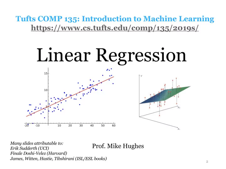
Tufts COMP 135: Introduction to Machine Learning https://www.cs.tufts.edu/comp/135/2019s/ Linear Regression Many slides attributable to: Prof. Mike Hughes Erik Sudderth (UCI) Finale Doshi-Velez (Harvard) James, Witten, Hastie, Tibshirani
Tufts COMP 135: Introduction to Machine Learning https://www.cs.tufts.edu/comp/135/2019s/ Linear Regression Many slides attributable to: Prof. Mike Hughes Erik Sudderth (UCI) Finale Doshi-Velez (Harvard) James, Witten, Hastie, Tibshirani (ISL/ESL books) 2
Objectives for Today (day 03) • Training “least squares” linear regression • Simplest case: 1-dim. features without intercept • Simple case: 1-dim. features with intercept • General case: Many features with intercept • Concepts (algebraic and graphical view) • Where do formulas come from? • When are optimal solutions unique? • Programming: • How to solve linear systems in Python • Hint: use np.linalg.solve ; avoid np.linalg.inv Mike Hughes - Tufts COMP 135 - Spring 2019 3
What will we learn? Evaluation Supervised Training Learning Data, Label Pairs Performance { x n , y n } N measure Task n =1 Unsupervised Learning data label x y Reinforcement Learning Prediction Mike Hughes - Tufts COMP 135 - Spring 2019 4
Task: Regression y is a numeric variable Supervised e.g. sales in $$ Learning regression y Unsupervised Learning Reinforcement Learning x Mike Hughes - Tufts COMP 135 - Spring 2019 5
Visualizing errors Mike Hughes - Tufts COMP 135 - Spring 2019 6
Evaluation Metrics for Regression N 1 • mean squared error X y n ) 2 ( y n − ˆ N n =1 N • mean absolute error 1 X | y n − ˆ y n | N n =1 Today, we’ll focus on mean squared error (MSE). Mean squared error is smooth everywhere . Good analytical properties and widely studied. Thus, it is a common choice. NB: Many applications, absolute error (or other error metrics) may be more suitable, if computational or analytical convenience was not the chief concern. Mike Hughes - Tufts COMP 135 - Spring 2019 7
<latexit sha1_base64="GH0G5C3UmjNZ9rLMU3vQwo9X1u4=">ACD3icbVC7TsNAEDyHVwgvAyXNiQgUmsgOSFBG0FAGiTykOLOl0tyvls7taQyMof0PArNBQgREtLx9weRSQMNJKo5ld7e4EseAaHOfbyiwtr6yuZdzG5tb2zv27l5NR4mirEojEalGQDQTXLIqcBCsEStGwkCwetC/Gv1e6Y0j+QtDGPWCklX8g6nBIzk28dej0A6HBUGPj/BHihOZFewO/yAPdqOA/8lLsj3847RWcCvEjcGcmjGSq+/eW1I5qETAIVROum68TQSokCTgUb5bxEs5jQPumypqGShEy30sk/I3xklDbuRMqUBDxRf0+kJNR6GAamMyTQ0/PeWPzPaybQuWilXMYJMEmnizqJwBDhcTi4zRWjIaGEKq4uRXTHlGEgokwZ0Jw519eJLVS0T0tlm7O8uXLWRxZdIAOUQG56ByV0TWqoCqi6BE9o1f0Zj1ZL9a79TFtzVizmX30B9bnD38YnE8=</latexit> Linear Regression 1-dim features, no bias Parameters: Graphical interpretation: Pick a line with slope w that goes through the origin w = [ weight scalar w = 1.0 Prediction: y ( x i ) , w · x i 1 w = 0.5 ˆ w = 0.0 Training : Input : training set of N observed examples of features x and responses y Output: value of w that minimizes mean squared error on training set. Mike Hughes - Tufts COMP 135 - Spring 2019 8
<latexit sha1_base64="kRNCTsnOS4C+Me5ga0rZgQRdjc4=">ACK3icbVDLSgMxFM34tr6qLt1cLEIFLTNV0I0gdeNKVKwKnTpk0tQGk8yQZNRhmH6PG3/FhS584Nb/MK1d+DoQOJxzLzfnhDFn2rjuqzM0PDI6Nj4xWZianpmdK84vnOoUYTWScQjdR5iTmTtG6Y4fQ8VhSLkNOz8Gqv59dU6VZJE9MGtOmwJeStRnBxkpBseYLJoPsBnwmwRfYdMIwO85z6HbB14kIMrnj5RcHUE4DCevgd7DJ0rx8G8g1uFmF1YtqUCy5FbcP+Eu8ASmhAQ6D4qPfikgiqDSEY60bnhubZoaVYTvOAnmsaYXOFL2rBUYkF1M+tnzWHFKi1oR8o+aCvft/IsNA6FaGd7KXRv72e+J/XSEx7u5kxGSeGSvJ1qJ1wMBH0ioMWU5QYnlqCiWL2r0A6WGFibL0FW4L3O/JfclqteBuV6tFmabc2qGMCLaFlVEYe2kK7aB8dojoi6A49oGf04tw7T86b8/41OuQMdhbRDzgfnwalpjs=</latexit> <latexit sha1_base64="RyMrO0KJWM2mqkB4hbk2yqhfto=">ACInicbZDLSsNAFIYn9VbrLerSzWARxEVJqAuCkU3rqSCvUCThsl0g6dTMLMRC0hz+LGV3HjQlFXg/j9LQ1h8O/HznHGbO78eMSmVZX0ZuYXFpeSW/Wlhb39jcMrd3GjJKBCZ1HLFItHwkCaOc1BVjLRiQVDoM9L0B5ejfvOCEkjfquGMXFD1OM0oBgpjTz/L5zBCvQCQTCKXRkEnopr9hZ5xoOPQ4fdGUzXLNOGWaeWbRK1lhw3thTUwRT1Tzw+lGOAkJV5ghKdu2FSs3RUJRzEhWcBJYoQHqEfa2nIUEum4xMzeKBJFwaR0MUVHNPfGykKpRyGvp4MkerL2d4I/tdrJyo4c1PK40QRjicPBQmDKoKjvGCXCoIVG2qDsKD6rxD3kU5L6VQLOgR79uR50yiX7ONS+eakWL2YxpEHe2AfHAIbnIquAI1UAcYPIJn8ArejCfjxXg3PiejOWO6swv+yPj+AehWoq0=</latexit> Training for 1-dim, no-bias LR Training objective: minimize squared error (“least squares” estimation) N X y ( x n , w )) 2 min ( y n − ˆ w ∈ R n =1 Formula for parameters that minimize the objective: P N n =1 y n x n w ∗ = P N n =1 x 2 n When can you use this formula? When you observe at least 1 example with non-zero features Otherwise, all possible w values will be perfect (zero training error) Why ? all lines in our hypothesis space go through origin. How to derive the formula (see notes): 1. Compute gradient of objective, as a function of w 2. Set gradient equal to zero and solve for w Mike Hughes - Tufts COMP 135 - Spring 2019 9
For details, see derivation notes https://www.cs.tufts.edu/comp/135/2020f/note s/day03_linear_regression.pdf Mike Hughes - Tufts COMP 135 - Spring 2019 10
<latexit sha1_base64="3CvL/Hb4nFjYE+qiVY/5uVs/3Q=">ACE3icbVDLSgNBEJz1GeNr1aOXwSBEhbAbBT0GvXiMYB6QDcvsZJIMmZ1dZ3o1Yck/ePFXvHhQxKsXb/6Nk8dBEwsaiqpuruCWHANjvNtLSwuLa+sZtay6xubW9v2zm5VR4mirEIjEal6QDQTXLIKcBCsHitGwkCwWtC7Gvm1e6Y0j+QtDGLWDElH8janBIzk28del0A6GOb7Pj/CHihOZEewO/yAPdqKAPf9lLtDfID3845BWcMPE/cKcmhKcq+/eW1IpqETAIVROuG68TQTIkCTgUbZr1Es5jQHumwhqGShEw30/FPQ3xolBZuR8qUBDxWf0+kJNR6EAamMyTQ1bPeSPzPayTQvmimXMYJMEkni9qJwBDhUC4xRWjIAaGEKq4uRXTLlGEgokxa0JwZ1+eJ9ViwT0tFG/OcqXLaRwZtI8OUB656ByV0DUqowqi6BE9o1f0Zj1ZL9a79TFpXbCmM3voD6zPH4SQnUQ=</latexit> <latexit sha1_base64="YJjhR7RY5hyNtVLBH/MermOQ7I=">AB6HicbVBNS8NAEJ3Ur1q/qh69LBbBU0mqoMeiF48t2FpoQ9lsJ+3azSbsboQS+gu8eFDEqz/Jm/GbZuDtj4YeLw3w8y8IBFcG9f9dgpr6xubW8Xt0s7u3v5B+fCoreNUMWyxWMSqE1CNgktsGW4EdhKFNAoEPgTj25n/8IRK81jem0mCfkSHkoecUWOlZtAvV9yqOwdZJV5OKpCj0S9/9QYxSyOUhgmqdzE+NnVBnOBE5LvVRjQtmYDrFrqaQRaj+bHzolZ1YZkDBWtqQhc/X3REYjrSdRYDsjakZ62ZuJ/3nd1ITXfsZlkhqUbLEoTAUxMZl9TQZcITNiYglitbCRtRZmx2ZRsCN7y6ukXat6F9Va87JSv8njKMIJnMI5eHAFdbiDBrSAcIzvMKb8+i8O/Ox6K14OQzx/AHzucPxi+M6g=</latexit> Linear Regression 1-dim features, with bias Parameters: Graphical interpretation: Predict along line with slope w and intercept b w = [ weight scalar w = 1.0 b = 0.0 b bias scalar Prediction: w = - 0.2 b = 0.6 y ( x i ) , w · x i 1 + b ˆ Training : Input : training set of N observed examples of features x and responses y Output: values of w and b that minimize mean squared error on training set. Mike Hughes - Tufts COMP 135 - Spring 2019 11
<latexit sha1_base64="U9/jy4ZC90GpwtZMYXOB0GAeOfg=">ACTHicbVDPSxtBGJ1NW6vpD1N7OWjoRDBht0otJeCtJeiopRIROX2clsMjgzu8x8W12W9f/rpYfe+lf04kERwUnMQWMfDze+x7fC/JlXQYhn+DxpOnz5aeL680X7x89Xq19WbtwGWF5aLPM5XZo4Q5oaQRfZSoxFuBdOJEofJybepf/hTWCczs49lLoajY1MJWfopbjFqZYmrk6BSgNUM5wkSbVXb0CyoNRwfg7UFTquzJeoPv4BVIkUO1DGBj4CnTCsyrpzFpsNOPXxdaBWjie4ftyLW+2wG84Aj0k0J20yx07c+kNHGS+0MgVc24QhTkOK2ZRciXqJi2cyBk/YWMx8NQwLdywmpVRwevjCDNrH8GYabeT1RMO1fqxE9Oj3OL3lT8nzcoMP08rKTJCxSG3y1KCwWYwbRZGEkrOKrSE8at9H8FPmGWcfT9N30J0eLJj8lBrxtdnu7W+3tr/M6lsk78p50SEQ+kW3yneyQPuHkF/lHLslV8Du4CK6Dm7vRjDPvCUP0Fi6BRF1sgo=</latexit> Training for 1-dim, with-bias LR Training objective: minimize squared error (“least squares” estimation) N y ( x n , w, b )) 2 X min ( y n − ˆ w ∈ R ,b ∈ R n =1 Formula for parameters that minimize the objective: P N n =1 ( x n − ¯ x )( y n − ¯ y ) w = x = mean( x 1 , . . . x N ) ¯ P N n =1 ( x n − ¯ x ) 2 y = mean( y 1 , . . . y N ) ¯ b = ¯ y − w ¯ x When can you use this formula? When you observe at least 2 examples with distinct 1-dim. features Otherwise, many w, b will be perfect (lowest possible training error) Why ? many lines in our hypothesis space go through one point How to derive the formula (see notes): 1. Compute gradient of objective wrt w, as a function of w and b 2. Compute gradient of objective wrt b, as a function of w and b 3. Set (1) and (2) equal to zero and solve for w and b (2 equations, 2 unknowns) Mike Hughes - Tufts COMP 135 - Spring 2019 12
Recommend
More recommend
Explore More Topics
Stay informed with curated content and fresh updates.
