LINEAR REGRESSION Sylvain Calinon Robot Learning & Interaction - PowerPoint PPT Presentation
EE613 Machine Learning for Engineers LINEAR REGRESSION Sylvain Calinon Robot Learning & Interaction Group Idiap Research Institute Nov. 4, 2015 1 Outline Multivariate ordinary least squares Singular value decomposition (SVD)
EE613 Machine Learning for Engineers LINEAR REGRESSION Sylvain Calinon Robot Learning & Interaction Group Idiap Research Institute Nov. 4, 2015 1
Outline • Multivariate ordinary least squares • Singular value decomposition (SVD) • Kernels in least squares (nullspace projection) • Ridge regression (Tikhonov regularization) • Weighted least squares (WLS) • Recursive least squares (RLS) 2
Multivariate ordinary least squares demo_LS01.m demo_LS_polFit01.m 3
Multivariate ordinary least squares • Least squares is everywhere: from simple problems to large scale problems. • It was the earliest form of regression, which was published by Legendre in 1805 and by Gauss in 1809. • They both applied the method to the problem of determining the orbits of bodies around the Sun from astronomical observations. • The term regression was only coined later by Galton to describe the biological phenomenon that the heights of descendants of tall ancestors tend to regress down towards a normal average (a phenomenon also known as regression toward the mean). • Pearson later provided the statistical context showing that the phenomenon is more general than a biological context.
Multivariate ordinary least squares Moore-Penrose pseudoinverse 5
Multivariate ordinary least squares 6
Multivariate ordinary least squares
Multivariate ordinary least squares 8
Least squares with Cholesky decomposition 9
Singular value decomposition (SVD) Matrix with non-negative diagonal entries (singular values of X) Unitary matrix Unitary matrix (orthonormal (orthonormal bases) bases)
Singular value decomposition (SVD) 11
Singular value decomposition (SVD) 12
Singular value decomposition (SVD) Applications employing SVD include pseudoinverse computation, least • squares fitting, multivariable control, matrix approximation, as well as the determination of the rank, range and null space of a matrix . The SVD can also be thought of as decomposing a matrix into a • weighted, ordered sum of separable matrices (e.g., decomposition of an image processing filter into separable horizontal and vertical filters). It is possible to use the SVD of a square matrix A to determine the • orthogonal matrix O closest to A . The closeness of fit is measured by the Frobenius norm of O − A . The solution is the product UV T . A similar problem, with interesting applications in shape analysis, is the • orthogonal Procrustes problem , which consists of finding an orthogonal matrix O which most closely maps A to B . Extensions to higher order arrays exist, generalizing SVD to a multi-way • analysis of the data (multilinear algebra). 13
Condition number of a matrix with SVD 14
Least squares with SVD 15
Least squares with SVD 16
Different line fitting alternatives 17
Data fitting with linear least squares • In linear least squares, we are not restricted to using a line as the model as in the previous slide! • For instance, we could have chosen a quadratic model Y=X 2 A: This model is still linear in the A parameter. The function does not need to be linear in the argument : only in the parameters that are determined to give the best fit. • Also, not all of X contains information about the datapoints: the first/last column can for example be populated with ones, so that an offset is learned • This can be used for polynomial fitting by treating x, x2, ... as being distinct independent variables in a multiple regression model. 18
Data fitting with linear least squares 19
Data fitting with linear least squares • Polynomial regression is an example of regression analysis using basis functions to model a functional relationship between two quantities. Specifically, it replaces x in linear regression with polynomial basis [ 1 , x , x 2 , … , x d ]. • A drawback of polynomial bases is that the basis functions are "non-local“. • It is for this reason that the polynomial basis functions are often used along with other forms of basis functions, such as splines, radial basis functions, and wavelets. (We will learn more about this at next lecture…) 20
Polynomial fitting with least squares 21
Kernels in least squares (nullspace projection) demo_LS_nullspace01.m 22
Kernels in least squares (nullspace) 23
Kernels in least squares (nullspace) 24
Kernels in least squares (nullspace) 25
Kernels in least squares (nullspace) without nullspace with nullspace 26
Example with polynomial fitting 27
Example with robot inverse kinematics Joint space / configuration space coordinates Task space / operational space coordinates 28
Example with robot inverse kinematics Keeping the tip still as primary constraint Trying to move the first joint as secondary constraint 29
Example with robot inverse kinematics Tracking target with right hand if possible Tracking target with left hand 30
Ridge regression (Tikhonov regularization, penalized least squares) demo_LS_polFit02.m 31
Ridge regression (Tikhonov regularization) 32
Ridge regression (Tikhonov regularization) 33
Ridge regression (Tikhonov regularization) 34
Ridge regression (Tikhonov regularization) 35
Ridge regression (Tikhonov regularization) 36
Ridge regression (Tikhonov regularization) 37
LASSO (L 1 regularization) • An alternative regularized version of least squares is Lasso (least absolute shrinkage and selection operator) using the constraint that the L 1 -norm |A| 1 is no greater than a given value. • The L 1 -regularized formulation is useful due to its tendency to prefer solutions with fewer nonzero parameter values, effectively reducing the number of variables upon which the given solution is dependent. • The increase of the penalty term in ridge regression will reduce all parameters while still remaining non-zero, while in Lasso, it will cause more and more of the parameters to be driven to zero . This is an advantage of Lasso over ridge regression, as driving parameters to zero deselects the features from the regression . 38
LASSO (L 1 regularization) • Thus, Lasso automatically selects more relevant features and discards the others, whereas ridge regression never fully discards any features. • Lasso is equivalent to an unconstrained minimization of the least-squares penalty with |A| 1 added. In a Bayesian context, this is equivalent to placing a zero-mean Laplace prior distribution on the parameter vector. • The optimization problem may be solved using quadratic programming or more general convex optimization methods, as well as by specific algorithms such as the least angle regression algorithm . 39
Weighted least squares (Generalized least squares) demo_LS_weighted01.m 40
Weighted least squares 41
Weighted least squares 42
Weighted least squares - Example 43
Weighted least squares - Example 44
Iteratively reweighted least squares (IRLS) demo_LS_IRLS01.m 45
Robust regression Regression analysis seeks to find the relationship between one • or more independent variables and a dependent variable. Methods such as ordinary least squares have favorable properties if their underlying assumptions are true, but can give misleading results if those assumptions are not true Least squares estimates are highly sensitive to outliers . Robust regression methods are designed to be not overly • affected by violations of assumptions through the underlying data-generating process. It down-weights the influence of outliers, which makes their residuals larger and easier to identify. A simple approach to robust least squares fitting is to first do an • ordinary least squares fit, then identify the k data points with the largest residuals, omit these, perform the fit on the remaining data. 46
Robust regression Another simple method to estimate parameters in a regression • model that are less sensitive to outliers than the least squares estimates is to use least absolute deviations . An alternative parametric approach is to assume that the residuals • follow a mixture of normal distributions : A contaminated normal distribution in which the majority of observations are from a specified normal distribution, but a small proportion are from a normal distribution with much higher variance. Another approach to robust estimation of regression models is to • replace the normal distribution with a heavy-tailed distribution (e.g., t-distributions). Bayesian robust regression often relies on such distributions. 47
Recommend
More recommend
Explore More Topics
Stay informed with curated content and fresh updates.
