Linear Regression Fernando Brito e Abreu (fba@di.fct.unl.pt) - PDF document
Experimental Software Engineering Linear Regression Fernando Brito e Abreu (fba@di.fct.unl.pt) Universidade Nova de Lisboa (http://www.unl.pt) QUASAR Research Group (http://ctp.di.fct.unl.pt/QUASAR) Summary Purpose of regression?
Experimental Software Engineering – Linear Regression – Fernando Brito e Abreu (fba@di.fct.unl.pt) Universidade Nova de Lisboa (http://www.unl.pt) QUASAR Research Group (http://ctp.di.fct.unl.pt/QUASAR) Summary � Purpose of regression? � Residuals independence: Durbin-Watson test � Linear Regression - Purpose � Multiple regression model � First order linear model � Linear regression validation � Probabilistic linear relationship � Inference testing (Regression � Residuals ANOVA) � Least squares method � Assessing the influence of � Linear model assumptions each X � Normal Probability Plot and � Variable selection methods Residuals Plot � Goodness of fit 12-May-08 Experimental Software Engineering / Fernando Brito e Abreu 1
Purpose of regression? � To determine whether values of one or more variables are related to the response variable � To predict the value of one variable based on the value of one or more variables Definitions: � Dependent variable (aka response or endogenous) � The variable that is being predicted or explained � Independent variable (aka explanatory, regressor or exogenous) � The variable that is doing the predicting or explaining 12-May-08 Experimental Software Engineering / Fernando Brito e Abreu Correlation or Regression? � Use correlation if you are interested only in whether a relationship exists � Use regression if you are interested in: � building a mathematical model that can predict the response (dependent) variable � the relative effectiveness of several variables in predicting the response variable 12-May-08 Experimental Software Engineering / Fernando Brito e Abreu 2
Linear regression - purpose � Is there an association between the two variables? � Is defect density (DD) change related to code complexity (CC) change? � Estimation of impact � How much DD change occurs per CC unit change? � Prediction � If a program looses 20 CC units (e.g. by refactoring it), how much of a drop in DD can be expected? SPSS : Analyse / Regression / Linear 12-May-08 Experimental Software Engineering / Fernando Brito e Abreu First order linear model (aka simple regression model) � A deterministic mathematical model between y and x: y = β 0 + β 1 * x � Y Regression line � β 0 is the intercept with y axis, observation the point at which x = 0 Rise � β 1 is the angle of the line, the Run ratio of rise divided by the run � It measures the change in y for one unit of change in x intercept X 12-May-08 Experimental Software Engineering / Fernando Brito e Abreu 3
Probabilistic linear relationship � Relationship between x and y is not always exact � Observations do not always fall on a straight line � To accommodate this, we introduce a random error term referred to as epsilon: y = β 0 + β 1 * x + ε � ε reflects how individuals deviate from others with the same value of x 12-May-08 Experimental Software Engineering / Fernando Brito e Abreu Probabilistic linear relationship � The task of regression analysis then is to estimate the parameters b 0 and b 1 in the equation: ^ = b 0 + b 1 * x y so that the difference between y and is minimized ^ y This is called the estimated simple linear regression equation � Notes: Notes: � is the estimate for β 0 and is the estimate for β 1 � b 0 is the estimate for and b 1 is the estimate for ^ is the estimated (predicted) value of y y for a given for a given x x value. value. is the estimated (predicted) value of � � y 12-May-08 Experimental Software Engineering / Fernando Brito e Abreu 4
Residuals � The distance between each observation (red dot) and the solid Y Regression line line (estimated regression line) is called residual � Residuals are deviations due to the random error term residual � The regression line is determined by minimizing the sum of the observation squared residuals X 12-May-08 Experimental Software Engineering / Fernando Brito e Abreu Least squares method � Criterion: Choose b 0 and b 1 to minimize the squared sum of squared residuals S = Σ ( y i – b 0 − b 1 x i ) 2 The regression line is the one that minimizes the sum of the squared distances of each observation to that line Slope: ∑ Intercept: − − ( x x )( y y ) = − = − b b y y b x b x = i i b 0 1 ∑ 0 1 − 1 2 ( x x ) i 12-May-08 Experimental Software Engineering / Fernando Brito e Abreu 5
Linear model assumptions (1) � Y variable: � is continuous (measured at least on an interval scale) � X variables: � can be continuous or indicator variables (nominal / ordinal) � do not need to be normally distributed � Note: � this assumption is valid both for simple (one X) or multiple (several Xs) regression models 12-May-08 Experimental Software Engineering / Fernando Brito e Abreu Linear model assumptions (2) ε ~ N(0, σ ) � The probability distribution of the error is Normal with mean 0 � The variance is constant, finite and not depending on X values � The latter is called homoscedasticity propriety � Homoscedastic = Having equal statistical variances � [homo (same) + Greek skedastos ("able to be scattered“)] � Rephrasing: For each value of X there is a population of Y’s that are normally distributed with the same variability � The population means form a straight line � Each population has the same variance σ 2 12-May-08 Experimental Software Engineering / Fernando Brito e Abreu 6
12-May-08 Experimental Software Engineering / Fernando Brito e Abreu Normal Probability Plot � Normal Probability Plot compares the percent of errors falling in particular bins (e.g. deciles) to the percentage expected from Normal distribution � If regression assumption is met then the plot should look like a straight line 12-May-08 Experimental Software Engineering / Fernando Brito e Abreu 7
Residual Plot RES IDUA L P LOT 10 5 esidual 0 4 6 8 10 R -5 -10 C oding productivity � Allows to observe if residuals have: � a mean of zero � Observations will be evenly scattered on both sides of the line � a constant standard deviation (not dependent on X value) � Observations will evenly scattered horizontally (across the X axis) 12-May-08 Experimental Software Engineering / Fernando Brito e Abreu Linear model assumptions (3) � A final regression assumption is that residuals are independent � This is equivalent to say that for all possible pairs of X i , X j (i ≠ j; i,j = 1, …, n), the errors ε i , ε j are not autocorrelated, that is, their covariance is null � This assumption can be evaluated with the Durbin-Watson statistic that allows testing the following hypothesis: � H 0 : Cov( ε i , ε j ) = 0 (i ≠ j; I,j = 1, …, n) � residuals are not autocorrelated (they are independent) � H 1 : Cov( ε i , ε j ) <> 0 � residuals are autocorrelated (their covariance is not negligible) Note : The Durbin-Watson statistic ranges in value from 0 to 4 SPSS : Analyze /Regression /Linear /Statistics /Residuals /Durbin- Watson 12-May-08 Experimental Software Engineering / Fernando Brito e Abreu 8
Residuals independence: Durbin-Watson test � Hypothesis acceptance decision is performed by comparing the statistic observed value (d) with tabled critical values: upper (dU) and lower bounds (dL) � SPSS help includes tables by Savin and White for several values of α � Table entries are the sample size (n) and the number of independent variables (k) � Decision: � d < dL , we reject H 0 and accept H 1 � residuals are not independent (they are autocorrelated) � d > dU , we accept H 0 and reject H 1 � residuals are independent 12-May-08 Experimental Software Engineering / Fernando Brito e Abreu Durbin and Watson statistic � Example: � d = 1,723 (observed value of Durbin-Watson statistic) � sample size (n) = 71 � number of independent variables (k) = 2 � From Savin and White table for α = 0,01 (in SPSS): � dL (2, 70) = 1.400 � dU (2, 70) = 1.514 Conclusion: since d > dU, we accept H 0 and reject H 1 � Residuals are independent! The assumption is met ☺ 12-May-08 Experimental Software Engineering / Fernando Brito e Abreu 9
Multiple regression model � These are models of the type y = β 0 + β 1 * x 1 + β 2 * x 2 + … + β p * x p + ε � These models require that the independent variables are near to orthogonal (statistically uncorrelated) � Aka: Absence of multicolinearity SPSS : Analyse / Regression / Linear � Note: to compare the magnitude of the influences of each independent variable (x i ) we must consider the standardized coefficients (aka Beta coefficients ) 12-May-08 Experimental Software Engineering / Fernando Brito e Abreu How to detect collinearity problems? Method 1: Bivariate correlation analysis � � Collinearity problem: Correlations > 75% (typical criterion) � � This method is only indicative; VIF or Tolerance should also be used SPSS (M1) : Analyze / Descriptive Statistics / Crosstabs Method 2: Variance Inflation Factor (VIF) � � Collinearity problem: VIF > 5 (other authors consider 10) � Method 3: Tolerance (T=1/VIF) � � Collinearity problem: T < 0.2 (other authors consider 0.1) � SPSS (M2,M3) : Analyze / Regression / Linear / Statistics / Collinearity diagnostics 12-May-08 Experimental Software Engineering / Fernando Brito e Abreu 10
Recommend
More recommend
Explore More Topics
Stay informed with curated content and fresh updates.
