Linear Programming Illustration Courtesy: Kevin Wayne & Denis - PowerPoint PPT Presentation
CSC373 Week 6: Linear Programming Illustration Courtesy: Kevin Wayne & Denis Pankratov 373F20 - Nisarg Shah 1 Announcement ACM ICPC Qualification Round Oct 24, 3-8pm EST Sign up at: https://www.teach.cs.toronto.edu/~acm/
CSC373 Week 6: Linear Programming Illustration Courtesy: Kevin Wayne & Denis Pankratov 373F20 - Nisarg Shah 1
Announcement • ACM ICPC Qualification Round • Oct 24, 3-8pm EST • Sign up at: https://www.teach.cs.toronto.edu/~acm/ • Top 9 participants will be chosen to represent U of T at the regional contest (broken into three teams of 3 each) 373F20 - Nisarg Shah 2
Recap • Network flow ➢ Ford-Fulkerson algorithm o Ways to make the running time polynomial ➢ Correctness using max-flow, min-cut ➢ Applications: o Edge-disjoint paths o Multiple sources/sinks o Circulation o Circulation with lower bounds o Survey design o Image segmentation o Profit maximization 373F20 - Nisarg Shah 3
Brewery Example • A brewery can invest its inventory of corn, hops and malt into producing some amount of ale and some amount of beer ➢ Per unit resource requirement and profit of the two items are as given below Example Courtesy: Kevin Wayne 373F20 - Nisarg Shah 4
Brewery Example • Suppose it produces 𝐵 units of ale and 𝐶 units of beer • Then we want to solve this program: 373F20 - Nisarg Shah 5
Linear Function • 𝑔: ℝ 𝑜 → ℝ is a linear function if 𝑔 𝑦 = 𝑏 𝑈 𝑦 for some 𝑏 ∈ ℝ 𝑜 𝑈 3 𝑦 1 ➢ Example: 𝑔 𝑦 1 , 𝑦 2 = 3𝑦 1 − 5𝑦 2 = −5 𝑦 2 • Linear objective: 𝑔 • Linear constraints: ➢ 𝑦 = 𝑑 , where : ℝ 𝑜 → ℝ is a linear function and 𝑑 ∈ ℝ ➢ Line in the plane (or a hyperplane in ℝ 𝑜 ) ➢ Example: 5𝑦 1 + 7𝑦 2 = 10 373F20 - Nisarg Shah 6
Linear Function • Geometrically, 𝑏 is the normal vector of the line(or hyperplane) represented by 𝑏 𝑈 𝑦 = 𝑑 373F20 - Nisarg Shah 7
Linear Inequality • 𝑏 𝑈 𝑦 ≤ 𝑑 represents a “half - space” 373F20 - Nisarg Shah 8
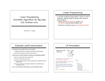
Linear Programming • Maximize/minimize a linear function subject to linear equality/inequality constraints 373F20 - Nisarg Shah 9
Geometrically… 373F20 - Nisarg Shah 10
Back to Brewery Example 373F20 - Nisarg Shah 11
Back to Brewery Example 373F20 - Nisarg Shah 12
Optimal Solution At A Vertex • Claim: Regardless of the objective function, there must be a vertex that is an optimal solution 373F20 - Nisarg Shah 13
Convexity • Convex set: 𝑇 is convex if 𝑦, 𝑧 ∈ 𝑇, 𝜇 ∈ [0,1] ⇒ 𝜇𝑦 + 1 − 𝜇 𝑧 ∈ 𝑇 • Vertex: A point which cannot be written as a strict convex combination of any two points in the set • Observation: Feasible region of an LP is a convex set 373F20 - Nisarg Shah 14
Optimal Solution At A Vertex • Intuitive proof of the claim: ➢ Start at some point 𝑦 in the feasible region ➢ If 𝑦 is not a vertex: o Find a direction 𝑒 such that points within a positive distance of 𝜗 from 𝑦 in both 𝑒 and −𝑒 directions are within the feasible region o Objective must not decrease in at least one of the two directions o Follow that direction until you reach a new point 𝑦 for which at least one more constraint is “tight” ➢ Repeat until we are at a vertex 373F20 - Nisarg Shah 15
LP, Standard Formulation • Input: 𝑑, 𝑏 1 , 𝑏 2 , … , 𝑏 𝑛 ∈ ℝ 𝑜 , 𝑐 ∈ ℝ 𝑛 ➢ There are 𝑜 variables and 𝑛 constraints • Goal: 373F20 - Nisarg Shah 16
LP, Standard Matrix Form • Input: 𝑑, 𝑏 1 , 𝑏 2 , … , 𝑏 𝑛 ∈ ℝ 𝑜 , 𝑐 ∈ ℝ 𝑛 ➢ There are 𝑜 variables and 𝑛 constraints • Goal: 373F20 - Nisarg Shah 17
Convert to Standard Form • What if the LP is not in standard form? ➢ Constraints that use ≥ o 𝑏 𝑈 𝑦 ≥ 𝑐 ⇔ −𝑏 𝑈 𝑦 ≤ −𝑐 ➢ Constraints that use equality o 𝑏 𝑈 𝑦 = 𝑐 ⇔ 𝑏 𝑈 𝑦 ≤ 𝑐, 𝑏 𝑈 𝑦 ≥ 𝑐 ➢ Objective function is a minimization o Minimize 𝑑 𝑈 𝑦 ⇔ Maximize −𝑑 𝑈 𝑦 ➢ Variable is unconstrained o 𝑦 with no constraint ⇔ Replace 𝑦 by two variables 𝑦 ′ and 𝑦 ′′ , replace every occurrence of 𝑦 with 𝑦 ′ − 𝑦 ′′ , and add constraints 𝑦 ′ ≥ 0, 𝑦 ′′ ≥ 0 373F20 - Nisarg Shah 18
LP Transformation Example 373F20 - Nisarg Shah 19
Optimal Solution • Does an LP always have an optimal solution? • No! The LP can “fail” for two reasons: 1. It is infeasible , i.e. 𝑦 𝐵𝑦 ≤ 𝑐} = ∅ o E.g. the set of constraints is 𝑦 1 ≤ 1, −𝑦 1 ≤ −2 2. It is unbounded , i.e. the objective function can be made arbitrarily large (for maximization) or small (for minimization) o E.g. “maximize 𝑦 1 subject to 𝑦 1 ≥ 0 ” • But if the LP has an optimal solution, we know that there must be a vertex which is optimal 373F20 - Nisarg Shah 20
Simplex Algorithm • Simple algorithm, easy to specify geometrically • Worst-case running time is exponential • Excellent performance in practice 373F20 - Nisarg Shah 21
Simplex: Geometric View 373F20 - Nisarg Shah 22
Algorithmic Implementation Move to a neighbor vertex with better objective value Start at a Is there a vertex of neighbor vertex feasible with better polytope objective value? Terminate, declare the current solution and value as optimal 373F20 - Nisarg Shah 23
How Do We Implement This? • We’ll work with the slack form of LP ➢ Convenient for implementing simplex operations ➢ We want to maximize 𝑨 in the slack form, but for now, forget about the maximization objective 373F20 - Nisarg Shah 24
Slack Form 373F20 - Nisarg Shah 25
Slack Form 373F20 - Nisarg Shah 26
Simplex: Step 1 • Start at a feasible vertex ➢ How do we find a feasible vertex? ➢ For now, assume 𝑐 ≥ 0 (each 𝑐 𝑗 ≥ 0 ) o In this case, 𝑦 = 0 is a feasible vertex. o In the slack form, this means setting the nonbasic variables to 0 ➢ We’ll later see what to do in the general case 373F20 - Nisarg Shah 27
Simple: Step 2 • What next? Let’s look at an example • To increase the value of 𝑨 : ➢ Find a nonbasic variable with a positive coefficient o This is called an entering variable ➢ See how much you can increase its value without violating any constraints 373F20 - Nisarg Shah 28
Simple: Step 2 This is because the current values of 𝑦 2 and 𝑦 3 are 0 , and we need 𝑦 4 , 𝑦 5 , 𝑦 6 ≥ 0 373F20 - Nisarg Shah 29
Simple: Step 2 Tightest obstacle ➢ Solve the tightest obstacle for the nonbasic variable 𝑦 1 = 9 − 𝑦 2 4 − 𝑦 3 2 − 𝑦 6 4 o Substitute the entering variable (called pivot) in other equations o Now 𝑦 1 becomes basic and 𝑦 6 becomes non-basic o 𝑦 6 is called the leaving variable 373F20 - Nisarg Shah 30
Simplex: Step 2 • After one iteration of this step: ➢ The basic feasible solution (i.e. substituting 0 for all nonbasic variables) improves from 𝑨 = 0 to 𝑨 = 27 • Repeat! 373F20 - Nisarg Shah 31
Simplex: Step 2 373F20 - Nisarg Shah 32
Simplex: Step 2 373F20 - Nisarg Shah 33
Simplex: Step 2 • There is no leaving variable (nonbasic variable with positive coefficient). • What now? Nothing! We are done. • Take the basic feasible solution ( 𝑦 3 = 𝑦 5 = 𝑦 6 = 0 ). • Gives the optimal value 𝑨 = 28 • In the optimal solution, 𝑦 1 = 8 , 𝑦 2 = 4, 𝑦 3 = 0 373F20 - Nisarg Shah 34
Simplex Overview Move to a neighbor vertex with better objective value Start at a Is there a vertex of neighbor vertex feasible with better polytope objective value? Terminate, declare the current solution and value as optimal 373F20 - Nisarg Shah 35
Simplex Overview Move to a neighbor vertex with better objective value Is there a Assuming 𝑐 ≥ neighbor vertex 0 , start with a basic feasible with better solution objective value? Terminate, declare the current solution and value as optimal 373F20 - Nisarg Shah 36
Simplex Overview Move to a neighbor vertex with better objective value Assuming 𝑐 ≥ Is there an 0 , start with a entering variable basic feasible with positive solution coefficient? Terminate, declare the current solution and value as optimal 373F20 - Nisarg Shah 37
Simplex Overview Pivot on a leaving variable Assuming 𝑐 ≥ Is there an 0 , start with a entering variable basic feasible with positive solution coefficient? Terminate, declare the current solution and value as optimal 373F20 - Nisarg Shah 38
Simplex Overview Pivot on a leaving variable Assuming 𝑐 ≥ Is there an 0 , start with a entering variable basic feasible with positive solution coefficient? Terminate, declare optimal value 373F20 - Nisarg Shah 39
Some Outstanding Issues • What if the entering variable has no upper bound? ➢ If it doesn’t appear in any constraints, or only appears in constraints where it can go to ∞ ➢ Then 𝑨 can also go to ∞ , so declare that LP is unbounded • What if pivoting doesn’t change the constant in 𝑨 ? ➢ Known as degeneracy , and can lead to infinite loops ➢ Can be prevented by “perturbing” 𝑐 by a small random amount in each coordinate ➢ Or by carefully breaking ties among entering and leaving variables, e.g., by smallest index (known as Bland’s rule ) 373F20 - Nisarg Shah 40
Recommend
More recommend
Explore More Topics
Stay informed with curated content and fresh updates.
