Linear Classifiers and the Perceptron William Cohen February 4, - PDF document
Linear Classifiers and the Perceptron William Cohen February 4, 2008 1 Linear classifiers Lets assume that every instance is an n -dimensional vector of real numbers x R n , and there are only two possible classes, y = (+1) and y = (
Linear Classifiers and the Perceptron William Cohen February 4, 2008 1 Linear classifiers Let’s assume that every instance is an n -dimensional vector of real numbers x ∈ R n , and there are only two possible classes, y = (+1) and y = ( − 1), so every example is a pair ( x , y ). (Notation: I will use boldface to indicate vectors here, so x = � x 1 , . . . , x n � ). A linear classifier is a vector w that makes the prediction n � y = sign( ˆ w i x i ) i =1 1 If you remember your linear where sign( x ) = +1 if x ≥ 0 and sign( x ) = − 1 if x < 0. algebra this weighted sum of x i ’s is called the inner product of w and x and it’s usually written w · x , so this classifier can be written even more compactly as y = sign( w · x ) ˆ Visually, for a vector w , x · w is the distance of the result you get “if you project x onto w ” (see Figure 1). It might seem that representing examples as real-number vectors is somewhat constrain- ing. It seems fine if your attributes are numeric (e.g., “Temperature=72”) but what if you have an attribute “Outlook” with three possible discrete values “Rainy”, “Sunny”, and “Cloudy”? One answer is to replace this single attribute with three binary attributes: one that set to 1 when the outlook is rainy, and zero otherwise; one that set to 1 when the outlook is sunny, and zero otherwise; and one that set to 1 when the outlook is cloudy, and zero otherwise. So a dataset like the one below would be converted to examples in R 4 as shown: Outlook Temp PlayTennis? Day1 Rainy 85 No − → ( � 1 , 0 , 0 , 85 � , − 1) Day2 Sunny 87 No − → ( � 1 , 0 , 0 , 87 � , − 1) Day3 Cloudy 75 Yes − → ( � 0 , 0 , 1 , 75 � , +1) 1 This is a little different from the usual definition, where sign(0) = 0, but I’d rather not have to deal with the question of what to predict when � n i =1 w i x i = 0. 1
Figure 1: A geometric view of the inner product. Another answer, of course, is to abandon these discrete values and instead focus on numeric attributes—e.g., let “Outlook” be encoded as a real number representing the prob- ability of rain, so that Day2 would be encoded as � 0 . 01 , 87 � , where the 0 . 01 means a 1/100 chance of rain. However, encoding your examples as pure numeric vectors vectors has one small problem. As I’ve defined it, a linear classifier is doomed to predict ˆ y = 1 on a perfectly sunny day (Outlook=0) if the temperature is also zero—regardless of what weight vector w you pick, w ·� 0 , 0 � will be zero, and ˆ y will be one. Since zero-degree weather isn’t conducive to playing tennis, no matter how clear it is, we can add one more trick to our encoding of examples and add an extra dimension to each vector, with a value that is always one. Let’s label that extra dimension 0: then n n � � y = sign( w 0 x 0 + ˆ w i x i ) = sign( w 0 + w i x i ) (1) i =1 i =1 the second half of the equation holding because for every example x , x 0 = 1. This trick gives our linear classifier a bit more expressive power, and we can still write our classifier using the super-compact notation ˆ y = sign( wx ) if we like. The weight w 0 is sometimes called a bias term . 2
2 Naive Bayes is a linear classifer How do you learn a linear classifier? Well, you already know one way. To make things simple, I’ll assume that x is not just a real-valued vector, but is a binary vector, in the discussion below. You remember that Naive Bayes can be written as follows: n � y = argmax y P ( y | x ) = argmax y P ( x | y ) P ( y ) = argmax y ˆ P ( x i | y ) P ( y ) i =1 Since the log function is monotonic we can write this as � n n � � � y = argmax y log ˆ P ( x i | y ) P ( y ) = argmax y log P ( x i | y ) + log P ( y ) i =1 i =1 And if there are only two classes, y = +1 and y = − 1, we can write this as �� n � n � �� � � y = sign ˆ log P ( x i | Y =+1) + log P ( Y =+1) − log P ( x i | Y =-1) + log P ( Y =-1) i =1 i =1 which we can rearrange as � n � � y = sign ˆ (log P ( x i | Y =+1) − log P ( x i | Y =-1)) + (log P ( Y =+1) − log P ( Y =-1)) i =1 y , we can write this as 2 and if we use the fact that log x − log( y ) = log x � n � log P ( x i | Y =+1) P ( x i | Y =-1) + log P ( Y =+1) � y = sign ˆ (2) P ( Y =-1) i =1 This is starting to look a little more linear! To finish the job, let’s think about what this means. When we say log P ( x i | Y =+1 ) P ( x i | Y =-1 ) , we’re using that to describe a function of x i , which could be written out as log P ( X i =1 | Y =+1 ) if x i = 1 P ( X i =1 | Y =-1 ) log P ( x i | Y =+1) P ( x i | Y =-1) ≡ f ( x i ) ≡ (3) log P ( X i =0 | Y =+1 ) if x i = 0 P ( X i =0 | Y =-1 ) To make the next few equations uncluttered let’s define p i and q i as log P ( X i = 1 | Y =+1) p i ≡ P ( X i = 1 | Y =-1) log P ( X i = 0 | Y =+1) q i ≡ P ( X i = 0 | Y =-1) 2 As an aside, expressions like o = log P ( Y =+1 ) P ( Y =-1 ) are called log odds , and they mean something. If the logs are base 2 and o = 3, then the event Y =+1 is 2 3 = 8 times as likely as the event Y =-1, while if o = − 4 then the event Y =-1 is about 2 4 = 16 times as likely as the event Y =+1. 3
A slightly tricky way to get rid of the if-thens in Equation 3 is to write it as f ( x i ) ≡ x i p i + (1 − x i ) q i (This is essentially the same trick as Tom used in deriving the MLE for a binomial - do you see why?) This of course can be written as f ( x i ) = x i ( p i − q i ) + q i (4) and then plugging Equation 4 into Equation 2 we get � n � ( x i ( p i − q i ) + q i ) + log P ( Y =+1) � y = sign ˆ (5) P ( Y =-1) i =1 Now, we’re almost done. Let’s define w i = p i − q i and define : w i ≡ p i − q i q i + log P ( Y =+1) � w 0 ≡ P ( Y =-1) i where w 0 is that “bias term” we used in Equation 1. Now the Naive Bayes prediction from Equation 5 becomes n � y = sign( ˆ x i w i + w 0 ) i =1 Putting it all together: for binary vectors x ′ = � x 1 , . . . , x n � Naive Bayes can be imple- mented as a linear classifier, to be applied to the augmented example x = � x 0 = 1 , x 1 , . . . , x n � . The weight vector w has this form: log P ( X i = 1 | Y =+1) P ( X i = 1 | Y =-1) − log P ( X i = 0 | Y =+1) w i ≡ P ( X i = 0 | Y =-1) (log P ( X i = 0 | Y =+1) P ( X i = 0 | Y =-1) ) + log P ( Y =+1) � w 0 ≡ P ( Y =-1) i and the Naive Bayes classification is y = sign( w · x ) ˆ 3 Online learning for classification 3.1 Online learning Bayesian probability is the most-studied mathematical model of learning. But there are other models that also are experimentally successful, and give useful insight. Sometimes these models are also mathematically more appropriate: e.g., even if all the probabilistic assumptions are correct, a MAP estimate might not minimize prediction errors. 4
Another useful model is on-line learning. In this document, I’ll consider on-line learners that can do two things. The first is to make a prediction ˆ y on an example x , where ˆ y ∈ {− 1 , +1 } . The second is to update the learner’s state, by “accepting” a new example � x , y � . As some background, remember that if θ is the angle between x and u , cos θ = x · u | | x | || | u | | This is important if you’re trying to keep a picture in your mind of what all these dot- products mean. A special case is that x · u = | | x | | cos θ when | | u | | = 1. Basically this means that for unit-length vectors, when dot products are large, the angle between the vectors must be small—i.e., the vectors must point in the same direction. Now consider this game, played between two players A and B . Player A provides examples x 1 , . . . , x T for each round (chosen arbitrarily). In each round, B first makes a prediction ˆ y i (say, using a learner L ). Then A picks a label y i , arbitrarily, to assign to x i . If sign( y i ) � = sign(ˆ y i )...or if you prefer, if y i ˆ y i < 0...then B has made a mistake . A is trying to force B to make as many mistakes as possible. To make this reasonable, we need a few more constraints on what A is allowed to do, and what B will do. 3.2 The perceptron game Here’s one version of the online-learning game. There are three extra rules, to make the game “fair” for B . Margin γ . A must provide examples that can be separated with some vector u with margin γ > 0, ie ∃ u : ∀ ( x i , y i ) given by A , ( u · x ) y i > γ and furthermore, | | u | | = 1. To make sense of this, recall that if θ is the angle between x and u , then cos θ = x · u | | x | || | u | | so if | | u | | = 1 then | | x | | cos θ = x · u . In other words, x · u is exactly the result of projecting x onto vector u , and x · u > γ means that x is distance γ away from the hyperplane h that is perpendicular to u . This hyperplane h is the separating hyperplane. Notice that y ( x · u ) > γ means that x is distance γ away from h on the “correct” side of h . Radius R . A must provide examples “near the origin”, ie | 2 < R ∀ x i given by A , | | x | B ’s strategy. B uses this learning strategy. 1. B ’s initial guess is v 0 = 0 . 5
Recommend
More recommend
Explore More Topics
Stay informed with curated content and fresh updates.
