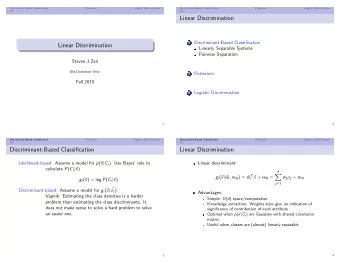
Linear Classification 1 / 14 The Linear Model In the next few - PowerPoint PPT Presentation
Linear Classification 1 / 14 The Linear Model In the next few lectures we will extend the perceptron learning algorithm to handle non-linearly separable data, explore online versis batch learning, learn three different learning
Linear Classification 1 / 14
The Linear Model In the next few lectures we will ◮ extend the perceptron learning algorithm to handle non-linearly separable data, ◮ explore online versis batch learning, ◮ learn three different learning settings – classification, regression, and probability estimation ◮ learn a fundamental concept in machine learning: gradient descent ◮ see how the learning rate hyperparameter 2 / 14
The Linear Model Recall that the linear model for binary classification is: w T · � H = { h ( � x ) = sign ( � x ) } where 1 w 0 w 1 x 1 ∈ R d +1 ∈ { 1 } × R d w = x = � � . . . . . . w d x d Where w ∈ R d +1 where d is the dimensionality of the input space and ◮ � w 0 is a bias weight, and ◮ x 0 = 1 is fixed. 3 / 14
Perceptron Learning Algorithm Recall the perceptron learning algorithm, slightly reworded: INPUT: a data set D with each � x i in D prepended with a 1, and labels � y 1. Initialize � w = ( w 0 , w 1 , ..., w d ) with zeros or random values, t = 1 w T · � 2. Receive a � x i ∈ D for which sign ( � x ) � = y i ◮ Update � w using the update rule: ◮ � w ( t + 1) ← � w ( t ) + y i � x i ◮ t ← t + 1 w T · � 3. If there is still a � x i ∈ D for which sign ( � x ) � = y i , repeat Step 2. TERMINATION: � w is a line separating the two classes (assuming D is linearly separable). Notice that the algorithm only updates the model based on a single sample. Such an algorithm is called an online learning algorithm. Also remember that PLA requires that D be linearly separable. 4 / 14
Two Fundamental Goals In Learning We have two fundamental goals with our learning algorithms: ◮ Make E out ( g ) close to E in ( g ) 1 . This means that our model will generallize well. We’ll learn how to bound the difference when we study computational learning theory. ◮ Make E in ( g ) small. This means we have a model that fits the data well, or performs well in its prediction task. Let’s now discuss how to make E in ( g ) small. We need to define small and we need to deal with non-separable data. 1 Remember that a version space is the set of all h in H consistent with our training data. g is the particular h chosen by the algorithm. 5 / 14
Non-Separable Data In practice perfectly linearly separable data is rare. Figure 1: Figure 3.1 from Learning From Data ◮ Data set could include noise which prevents linear separablility. ◮ Data might be fundamentally non-linearly separable. 6 / 14 Today we’ll learn how to deal with the first case. In a few days we’ll
Minimizing the Error Rate Earlier in the course we said that every machine learning problem contains the following elements: ◮ An input � x ◮ An unkown target function f : X → Y ◮ A data set D ◮ A learning model, which consists of ◮ a hypothesis class H from which our model comes, ◮ a loss function that quantifies the badness of our model, and ◮ a learning algorithm which optimizes the loss function. Error, E , is another term for loss function. For the case of our simple perceptron classifer we’re using 0-1 loss, that is, counting the errors (or proportion thereof) and our optmization procedure tries to find: N 1 w T � � min � sign ( � x n ) � = y n � N w ∈ R d +1 � n =1 Let’s look at two modifications to the PLA that perform this 7 / 14 minimization.
Batch PLA 2 INPUT: a data set D with each � x i in D prepended with a 1, labels � y , ǫ – an error tolerance, and α – a learning rate 1. Initialize � w = ( w 0 , w 1 , ..., w d ) with zeros or random values, t = 1, ∆ = (0 , .. 0) 2. do ◮ For i = 1 , 2 , ..., N w T · � ◮ if sign ( � x i ) � = y i , then ∆ ← ∆ + y i � x i ◮ ∆ ← ∆ N ◮ � w ← � w + α ∆ while || ∆ || 2 > ǫ TERMINATION: � w is “close enough” a line separating the two classes. 2 Based on Alan Fern via Byron Boots 8 / 14
New Concepts in the Batch PLA Algorithm 1. Initialize � w = ( w 0 , w 1 , ..., w d ) with zeros or random values, t = 1, ∆ = (0 , .. 0) 2. do ◮ For i = 1 , 2 , ..., N w T · � ◮ if sign ( � x i ) � = y i , then ∆ ← ∆ + y i � x i ◮ ∆ ← ∆ N ◮ � w ← � w + α ∆ while || ∆ || 2 > ǫ Notice a few new concepts in the batch PLA algorithm: ◮ the inner loop. This is a batch algorithm – it uses every sample in the data set to update the model. ◮ the ǫ hyperparameter – our stopping condition is “good enough”, i.e., within an error tolerance ◮ the α (also sometimes η ) hyperparameter – the learning rate, i.e., how much do we update the model in a given step. 9 / 14
Pocket Algorithm Input: a data set D with each � x i in D prepended with a 1, labels � y , and T steps 1. Initialize � w = ( w 0 , w 1 , ..., w d ) with zeros or random values, t = 1, ∆ = (0 , .. 0) 2. for t = 1 , 2 , ..., T ◮ Run PLA for one update to obtain � w ( t + 1) ◮ Evaluate E in ( � w ( t + 1)) ◮ if E in ( � w ( t + 1)) < E in ( � w ( t )), then � w ( t + 1) w ← � 3. On termination, � w is the best line found in T steps. Notice ◮ there is an inner loop under Step 2 to evaluate E in . This is also a batch algorithm – it uses every sample in the data set to update the model. ◮ the T hyperparameter simply sets a hard limit on the number of learning iterations we perform 10 / 14
Features Remember that the target function we’re trying to learn has the form f : X → Y , where X is typically a matrix of feature vectors and Y is a vector of corresponding labels (classes). Consider the problem of classifying images of hand-written digits: What should the feature vector be? 11 / 14
Feature Engineering Sometimes deriving descriptive features from raw data can improve the performance of machine learning algorithms. 3 Here we project the 256 features of the digit images (more if you consider pixel intensity) into a 2-dimensional space: average intensity and symmetry. 3 http://www.cs.rpi.edu/~magdon/courses/learn/slides.html 12 / 14
Multiclass Classification We’ve only discussed binary classifers so far. How can we deal with a multiclass problem, e.g., 10 digits? ◮ Some classifiers can do multi-class classification (e.g., multinomial logistic regression). ◮ Binary classifiers can be combined in a chain to handle multiclass problems This is a simple example of an ensemble, which we’ll discuss in greater detail in the second half of the course. 13 / 14
Closing Thoughts ◮ Most data sets are not linearly separable ◮ We minimize some error, or loss function ◮ Learning algorithms learn in one of two modes: ◮ Online learning algorithm – model is updated after seeing one training samples ◮ Batch learning algorithm – model is updated after seeing all training samples ◮ We’ve now seen hyperparamters to tune the operation of learning algorithms ◮ T or ǫ to bound the number of learning iterations ◮ A learning rate, α or η , to modulate the step size of the model update performed in each iteration ◮ A multiclass classification problem can be solved by a chain of binary classifiers 14 / 14
Recommend
More recommend
Explore More Topics
Stay informed with curated content and fresh updates.

![Classification Image Classification Set of predefined categories [eg: table, apple, dog, giraffe]](https://c.sambuz.com/743996/classification-s.webp)
