Linear classification Course of Machine Learning Master Degree in - PowerPoint PPT Presentation
Linear classification Course of Machine Learning Master Degree in Computer Science University of Rome Tor Vergata Giorgio Gambosi a.a. 2018-2019 1 Introduction 2 Classification most common case: disjoint classes, each input has
Linear classification Course of Machine Learning Master Degree in Computer Science University of Rome “Tor Vergata” Giorgio Gambosi a.a. 2018-2019 1
Introduction 2
Classification • most common case: disjoint classes, each input has to assigned to exactly one class • in linear classification models decision boundaries are linear functions feature space) • datasets such as classes correspond to regions which may be separated 3 • value t to predict are from a discrete domain, where each value denotes a class • input space is partitioned into decision regions of input x ( D − 1 -dimensional hyperplanes in the D -dimensional by linear decision boundaries are said linearly separable
Regression and classification • Classification: several ways to represent classes (target variable values) 4 • Regression: the target variable t is a vector of reals • Binary classification: a single variable t ∈ { 0 , 1 } , where t = 0 denotes class C 0 and t = 1 denotes class C 1 • K > 2 classes: “1 of K ” coding. t is a vector of K bits, such that for each class C j all bits are 0 except the j -th one (which is 1)
Approaches to classification Three general approaches to classification a class (decision phase) 3. generative approach: determine the class conditional distributions to assign an input to a class 5 1. find f : X �→ { 1 , . . . , K } (discriminant function) which maps each input x to some class C i (such that i = f ( x ) ) 2. discriminative approach: determine the conditional probabilities p ( C j | x ) (inference phase); use these distributions to assign an input to p ( x | C j ) , and the class prior probabilities p ( C j ) ; apply Bayes’ formula to derive the class posterior probabilities p ( C j | x ) ; use these distributions
Discriminative approaches • Approaches 1 and 2 are discriminative: they tackle the classification problem by deriving from the training set conditions (such as decision boundaries) that , when applied to a point, discriminate each class from the others • The boundaries between regions are specify by discrimination functions 6
Generalized linear models • In linear regression, a model predicts the target value; the prediction is functions could be applied) • In classification, a model predicts probabilities of classes, that is values 7 made through a linear function y ( x ) = w T x + w 0 (linear basis in [0 , 1] ; the prediction is made through a generalized linear model y ( x ) = f ( w T x + w 0 ) , where f is a non linear activation function with codomain [0 , 1] • boundaries correspond to solution of y ( x ) = c for some constant c ; this results into w T x + w 0 = f − 1 ( c ) , that is a linear boundary. The inverse function f − 1 is said link function.
Generative approaches • Approach 3 is generative: it works by defining, from the training set, a model of items for each class • The model is a probability distribution (of features conditioned by the class) and could be used for random generation of new items in the class • By comparing an item to all models, it is possible to verify the one that best fits 8
Discriminant functions 9
Linear discriminant functions in binary classification 10 • Decision boundary: D − 1 -dimensional hyperplane y ( x ) = 0 of all points s.t. w T x + w 0 = 0 • Given x 1 , x 2 on the hyperplane, y ( x 1 ) = y ( x 2 ) = 0 . Hence, w T ( x 1 ) − w T ( x 2 ) = w T ( x 1 − x 2 ) = 0 that is, x 1 − x 2 , w orthogonal • For any x s.t. y ( x ) = 0 , w T x is the length of the projection of x in the direction of w (orthogonal to the hyperplane y ( x ) = 0 ), in multiples of || w || 2 √∑ i w 2 • By normalizing wrt to || w || 2 = i , we get the length of the projection of x in the direction orthogonal to the hyperplane, assuming || w || 2 = 1 • Since w T x = − w 0 , w T x || w || = − w 0 || w || thus, the distance is determined by the threshold w 0
Linear discriminant functions in binary classification • The sign of the returned value discriminates in which of the regions separated by the hyperplane the point lies 11 • In general, for any x , y ( x ) = w T x + w 0 returns the distance (in multiples of || w || ) of x from the hyperplane
Linear discriminant functions in multiclass classification First approach 12 • Define K − 1 discrimination functions • Function f i ( 1 ≤ i ≤ K − 1 ) discriminates points belonging to class C i from points belonging to all other classes: if f i ( x ) > 0 then x ∈ C i , otherwise x ̸∈ C i • The green region belongs to both R 1 and R 2
Linear discriminant functions in multiclass classification Second approach classes • The green region is unassigned 13 • Define K ( K − 1) / 2 discrimination functions, one for each pair of • Function f ij ( 1 ≤ i < j ≤ K ) discriminates points which might belong to C i from points which might belong to C j • Item x is classified on a majority basis
Linear discriminant functions in multiclass classification Third approach 14 • Define K linear functions y i ( x ) = w T i x + w i 0 1 ≤ i ≤ K Item x is assigned to class C k iff y k ( x ) > y j ( x ) for all j ̸ = k : that is, k = argmax y j ( x ) j • Decision boundary between C i and C j : all points x s.t. y i ( x ) = y j ( x ) , a D − 1 -dimensional hyperplane ( w i − w j ) T x + ( w i 0 − w j 0 ) = 0
Linear discriminant functions in multiclass classification The resulting decision regions are connected and convex 15 • Given x A , x B ∈ R k then y k ( x A ) > y j ( x A ) and y k ( x B ) > y j ( x B ) , for all j ̸ = k • Let ˆ x = λ x A + (1 − λ ) x B , 0 ≤ λ ≤ 1 • For all i , since y i is linear for all, y i (ˆ x ) = λy i ( x a ) + (1 − λ ) y i ( x B ) • Then, y k (ˆ x ) > y j (ˆ x ) for all j ̸ = k ; that is, ˆ x ∈ R k R j R i R k x B x A � x
Generalized discriminant functions • The definition can be extended to include terms relative to products of boundaries can be more complex 16 pairs of feature values (Quadratic discriminant functions) D D i ∑ ∑ ∑ y ( x ) = w 0 + w i x i + w ij x i x j i =1 i =1 j =1 d ( d + 1) additional parameters wrt the d + 1 original ones: decision 2 • In general, generalized discrimination functions through set of functions φ i , . . . , φ m M ∑ y ( x ) = w 0 + w i φ i ( x ) i =1
Least squares and classification 17
Linear discriminant functions and regression • Group all parameters together as 18 • Assume classification with K classes • Classes are represented through a 1-of- K coding scheme: set of variables z 1 , . . . , z K , class C i coded by values z i = 1 , z k = 0 for k ̸ = i • Discriminant functions y i are derived as linear regression functions with variables z i as targets • To each variable z i a discriminant function y i ( x ) = w T i x + w i 0 is associated: x is assigned to the class C k s.t. k = argmax y i ( x ) i • Then, z k ( x ) = 1 and z j ( x ) = 0 ( j ̸ = k ) if k = argmax y i ( x ) i T x y ( x ) = W
Linear discriminant functions and regression • In general, a regression function provides an estimation of the target • In this case, dealing with a Bernoulli distribution, the expectation corresponds to the posterior probability 19 given the input E [ t | x ] • Value y i ( x ) can then be seen as a (poor) estimation of the conditional expectation E [ z i | x ] of variable z i given x ; hence, y i ( x ) is an estimate of p ( C i | x ) . However, y i ( x ) is not a probability E [ z i | x ] = P ( z i = 1 | x ) · 1 + P ( z i = 0 | x ) · 0 = P ( z i = 1 | x ) = P ( C i | x )
20 . . . . ... . . . . . Learning functions y i • Given a training set T , a regression function is derived by least squares R D e t i ∈ { 0 , 1 } K • An item in T is a pair ( x i , t i ) , x i ∈ I R ( D +1) × K is the matrix of parameters of all functions y i : the i -th • W ∈ I column represents the D + 1 parameters w i 0 , . . . , w iD of y i w 10 w 20 · · · w K 0 w 11 w 21 · · · w K 1 W = w 1 D w 2 D · · · w KD T x with x = (1 , x 1 , . . . , x d ) • y ( x ) = W
21 . . . . ... . . . . . set Learning functions y i R n × ( D +1) is the matrix of feature values for all items in the traing • X ∈ I x (1) x ( D ) 1 · · · 1 1 x (1) x ( D ) 1 · · · 2 2 X = x (1) x ( D ) 1 · · · n n • Then, for matrix XW , of size n × K , we have D ∑ x ( k ) ( XW ) ij = w j 0 + w jk = y j ( x i ) i k =1
22 Learning functions y i • y j ( x i ) is compared to item T ij in the matrix T , of size n × K , of target values, where row i is the 1-of- K coding of the class of item x i ( XW − T ) ij = y j ( x i ) − t ij • Let us consider the diagonal items of ( XW − T ) T ( XW − T ) . Then, K (( XW − T ) T ( XW − T )) ii = ∑ ( y j ( x i ) − t ij ) 2 j =1 That is, assuming x i is in class C k , (( XW − T ) T ( XW − T )) ii = ( y k ( x i ) − 1) 2 + ∑ y j ( x i ) 2 j ̸ = k
have to minimize: between observed values and values computed by the model, with • Standard approach, solve 23 Learning functions y i • Summing all elements on the diagonal of ( XW − T ) T ( XW − T ) provides the overall sum, on all items in T , of squared differences parameters W • This corresponds to the trace of ( XW − T ) T ( XW − T ) . Hence, we E ( W ) = 1 2 tr (( XW − T ) T ( XW − T )) ∂E ( W ) = 0 ∂ W
Recommend
More recommend
Explore More Topics
Stay informed with curated content and fresh updates.



![Classification Image Classification Set of predefined categories [eg: table, apple, dog, giraffe]](https://c.sambuz.com/743996/classification-s.webp)
