Lecture outline Introduction to the course Introduction to Machine - PowerPoint PPT Presentation
1 Introduction to Machine Learning Lecture 1: Introduction and Linear Regression Iasonas Kokkinos Iasonas.kokkinos@gmail.com University College London 2 Lecture outline Introduction to the course Introduction to Machine Learning Least
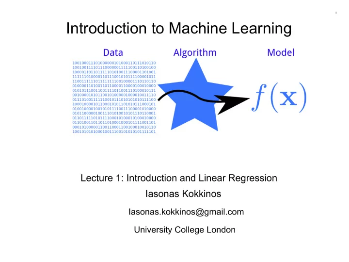
1 Introduction to Machine Learning Lecture 1: Introduction and Linear Regression Iasonas Kokkinos Iasonas.kokkinos@gmail.com University College London
2 Lecture outline Introduction to the course Introduction to Machine Learning Least squares
3 Machine Learning Principles, methods, and algorithms for learning and prediction based on past evidence Goal: Machines that perform a task based on experience, instead of explicitly coded instructions Why? • Crucial component of every intelligent/autonomous system • Important for a system’s adaptability • Important for a system’s generalization capabilities • Attempt to understand human learning
4 Machine Learning variants • Supervised – Classification – Regression • Unsupervised – Clustering – Dimensionality Reduction • Weakly supervised/semi-supervised Some data supervised, some unsupervised • Reinforcement learning Supervision: sparse reward for a sequence of decisions
5 Classification • Based on our experience, should we give a loan to this customer? – Binary decision: yes/no Decision boundary
6 Classification examples • Digit Recognition • Spam Detection • Face detection
7 `Faceness function’: classifier Decision boundary Background Face
8 Test time: deploy the learned function • Scan window over image – Multiple scales – Multiple orientations • Classify window as either: – Face – Non-face Face Window Classifier Non-face
9 Machine Learning variants • Supervised – Classification – Regression • Unsupervised – Clustering – Dimensionality Reduction • Weakly supervised Some data supervised, some unsupervised • Reinforcement learning Supervision: reward for a sequence of decisions
10 Regression • Output: Continuous – E.g. price of a car based on years, mileage, condition, …
11 Computer vision example • Human estimation: from image to vector-valued pose estimate
12 Machine Learning variants • Supervised – Classification – Regression • Unsupervised – Clustering – Dimensionality Reduction • Weakly supervised Some data supervised, some unsupervised • Reinforcement learning Supervision: reward for a sequence of decisions
13 Clustering • Break a set of data into coherent groups – Labels are `invented’
14 Clustering examples • Spotify recommendations
15 Clustering examples • Image segmentation
16 Machine Learning variants • Supervised – Classification – Regression • Unsupervised – Clustering – Dimensionality Reduction • Weakly supervised Some data supervised, some unsupervised • Reinforcement learning Supervision: reward for a sequence of decisions
17 Dimensionality reduction & manifold learning • Find a low-dimensional representation of high-dimensional data – Continuous outputs are `invented’
18 Example of nonlinear manifold: faces Average of two faces is not a face 1 2( x 1 + x 2 ) x 2
19 Moving along the learned face manifold Trajectory along the “male” dimension Trajectory along the “young” dimension Lample et. al. Fader Networks, NIPS 2017
20 Machine Learning variants • Supervised – Classification – Regression • Unsupervised – Clustering – Dimensionality Reduction • Weakly supervised/semi supervised Partially supervised • Reinforcement learning Supervision: reward for a sequence of decisions
21 Weakly supervised learning: only part of the supervision signal Supervision signal: “motorcycle” Inferred localization information
22 Weakly supervised learning: only part of the supervision signal Supervision signal: “motorcycle” Inferred localization information
23 Semi-supervised learning: only part of the data labelled Labelled data Labelled + unlabelled data
24 Machine Learning variants • Supervised – Classification – Regression • Unsupervised – Clustering – Dimensionality Reduction • Weakly supervised/semi supervised learning Some data supervised, some unsupervised • Reinforcement learning Supervision: reward for a sequence of decisions
25 Reinforcement learning • Agent interacts with environment repeatedly – Take actions, based on state – (occasionally) receive rewards – Update state – Repeat • Goal: maximize cumulative reward
26 Reinforcement learning examples • Beat human champions in games Backgammon, 90’s GO, 2015 • Robotics
27 Focus of first part: supervised learning • Supervised – Classification – Regression • Unsupervised – Clustering – Dimensionality Reduction, Manifold Learning • Weakly supervised Some data supervised, some unsupervised • Reinforcement learning Supervision: reward for a sequence of decisions
28 Classification: yes/no decision
29 Regression: continuous output
30 What we want to learn: a function • Input-output mapping y = f w ( x )
31 What we want to learn: a function • Input-output mapping method prediction y = f w ( x ) Input parameters
32 What we want to learn: a function method prediction y = f w ( x ) Input parameters x ∈ R Calculus x ∈ R D Vector calculus Machine learning: can work also for discrete inputs, strings, trees, graphs, …
33 What we want to learn: a function method prediction y = f w ( x ) Input parameters y ∈ { 0 , 1 } Classification: y ∈ R Regression:
34 What we want to learn: a function method prediction y = f w ( x ) Linear classifiers, neural networks, decision trees, ensemble models, probabilistic classifiers, …
35 Example of method: K-nearest neighbor classifier X X X (a) 1-nearest neighbor (b) 2-nearest neighbor (c) 3-nearest neighbor – Compute distance to other training records – Identify K nearest neighbors – Take majority vote
36 Training data for NN classifier (in R 2 )
37 1-nn classifier prediction (in R 2 )
38 3-nn classifier prediction
39 Method example: decision tree Machine learning: can work also for discrete inputs, strings, trees, graphs, …
40 Method example: decision tree
41 Method example: decision tree What is the depth of the decision tree for this problem?
42 Method example: linear classifier Feature coordinate j Feature coordinate i
43 Method example: neural network
44 Method example: neural network
45 Method example: neural network
46 We have two centuries of material to cover! https://en.wikipedia.org/wiki/Least_squares The first clear and concise exposition of the method of least squares was published by Legendre in 1805. The technique is described as an algebraic procedure for fitting linear equations to data and Legendre demonstrates the new method by analyzing the same data as Laplace for the shape of the earth. The value of Legendre's method of least squares was immediately recognized by leading astronomers and geodesists of the time
47 What we want to learn: a function • Input-output mapping method prediction y = f w ( x ) = f ( x ; w ) Input parameters w ∈ R w ∈ R K
48 Assumption: linear function y = f w ( x ) = f ( x , w ) = w T x Inner product: D X w T x = h w , x i = w d x d d =1 x ∈ R D , w ∈ R D
49 Reminder: linear classifier ⋅ + ≥ x positive : x w b 0 Feature coordinate j i i ⋅ + < x negative : x w b 0 i i Each data point has a class label: +1 ( ) y t = -1 ( ) Feature coordinate i
50 Question: which one? ⋅ + ≥ x positive : x w b 0 Feature coordinate j i i ⋅ + < x negative : x w b 0 i i Each data point has a class label: +1 ( ) y t = -1 ( ) Feature coordinate i
51 Linear regression in 1D
52 Linear regression in 1D Training set: input–output pairs S = { ( x i , y i ) } , i = 1 . . . , N x i ∈ R , y i ∈ R
53 Linear regression in 1D y i = w 0 + w 1 x i 1 + ✏ i = w 0 x i 0 + w 1 x i 1 + ✏ i , x i ∀ i 0 = 1 , = w T x i + ✏ i
54 Sum of squared errors criterion y i = w T x i + ✏ i Loss function: sum of squared errors N X ( ✏ i ) 2 L ( w ) = i =1 Expressed as a function of two variables: N �⇤ 2 X y i − w 0 x i 0 + w 1 x i ⇥ � L ( w 0 , w 1 ) = 1 i =1 Question: what is the best (or least bad) value of w? Answer: least squares
55 Calculus 101 f ( x ) x ∗ x
56 Calculus 101 f ( x ) x ∗ x x ∗ = argmax x f ( x )
57 Condition for maximum: derivative is zero f ( x ) x ∗ x x ∗ = argmax x f ( x )
58 Condition for maximum: derivative is zero f ( x ) x ∗ x x ∗ = argmax x f ( x ) f 0 ( x ⇤ ) = 0 →
59 Condition for minimum: derivative is zero x ∗ = argmin x f ( x ) f 0 ( x ⇤ ) = 0 →
60 Vector calculus 101 " # ∂ f f ( x ) ∂ x 1 f ( x ) = c r f ( x ) = ∂ f ∂ x 2 2D function graph isocontours gradient field r f ( x ) = 0 at minimum of function:
Recommend
More recommend
Explore More Topics
Stay informed with curated content and fresh updates.

