Lecture 8 - Signal and Image Processing - PowerPoint PPT Presentation
Lecture 8 - Signal and Image Processing NENS230:AnalysisTechniquesinNeuroscience Fall2015 Outline 1. Introduction to concepts in signal processing 2. The Fourier transform 3. Sampling frequency 4. Filtering 5. Image
Lecture 8 - Signal and Image Processing NENS�230:�Analysis�Techniques�in�Neuroscience� Fall�2015
Outline 1. Introduction to concepts in signal processing 2. The Fourier transform 3. Sampling frequency 4. Filtering 5. Image Processing 6. Audio read / write
What constitutes a ‘signal’ ? • Pretty much any measurement or piece of data… • Most common: values that vary across either time or space • Properties of signals: • dimensionality (1D, 2D, etc.) • sampling rate (samples per second) • range (max value - min value) • Some examples • Audio waveform from a microphone
Fourier Analysis: A primer Useful�for: • Noise Reduction • Period Estimation • Anti-aliasing • and much, much more ....
Fourier Analysis: A primer Time�Domain Frequency�Domain
Simple Signals
Simple Signals
Linearity
Linearity
Complex Signals
Demo: Fourier Series representation of a square wave
Fourier Analysis: A primer Time�Domain Fourier Inverse Fourier Transform Transform Frequency�Domain
The Fourier Transform • Decomposes a time series signal into a sum of sine and cosine signals of various amplitudes and frequencies. • Can be used to identify the dominant frequencies in a signal • Lots of mathematical depth we can’t go into here (there’s a whole Stanford course: EE261, The Fourier transform and its applications)
Fourier Analysis in Matlab Given�a�signal�y(t): F = fft(y); Computes�the�Fast�Fourier�Transform�(FFT)� F�is�a�vector�the�same�size�as�y
Demo: FFT on Audio Signal
Fourier Analysis in Matlab Excellent�toolbox�for�spectral�analysis: Chronux:�����www.chronux.org Example�uses:� 1) LFP�Analysis� 2) Spike-spike�coherence� 3) spike-field�coherence� 4) etc.
Nyquist limit You�can�only�resolve�or�estimate�frequencies�up�to�half� of�the�sampling�rate� •Note�that�rate�can�refer�to:� 1. Time�(e.g.:�audio�signal�sampling�rate)� 2. Space�(e.g.:�pixel�resolution�in�microscopy�image)� This�has�important�implications�for�your�data�collection.� You�have�to�sample�fast�enough�or�with�high�enough� spatial�resolution�to�capture�the�signals�of�interest.��
Sampling too slow
Demo: Sampling Frequency
Filtering • What should you do if you only care about a signal within a certain frequency band? • How to deal with noise? • If you know what you’re looking for (e.g.: neural spikes, LFP , some radio signal, bird chirp audio, etc) then you can filter out frequencies not contained in that signal • Conceptually similar to fluorescence microscopy (want to keep only specific frequencies and remove the rest).
Filtering Example Uses • Isolating neural spikes from LFP (or LFP from spikes) • Removing 60 Hz “hum” from electrical recordings • Removing background noise from audio recording • Almost any application involving quantitative measurement
Designing filters in Matlab • Again, there’s a lot of depth we can’t cover here, and whole courses designed around filtering math and theory. • Matlab hides much of this complexity and makes filter design relatively simple fdatool • Filter Design and Analysis tool
Demo: Filter Design
Signal Processing in Matlab Other�useful�functions�(see� documentation�for�more�info): filter (apply�a�filter�to�a�signal) conv (convolution) xcorr (cross�correlation)
Peak Detection Lots�of�different�algorithms,�we�will�use�one� on�FileExchange:
Image Processing • Many image processing algorithms are 2D generalizations of signal processing algorithms • Examples: (Gaussian blur = 2D convolution of filter coefficients 1. with an image) Affine image registration - 2D cross correlation 2. • Play around with the NUMEROUS demos if you’re interested in exploring image processing
Image Processing image filter * =
Image Processing Loading/Displaying�images: imread imshow rgb2gray Filtering�images: imfilter fspecial
Demo: Image Processing
Audio Reading�audio�files: [y, fs] = wavread(‘sound.wav’); % also see: audioread % use wavwrite to save audio Can�import�many�other�file�types,�like�.mp3� using�File�Exchange�importers.
Demo: Audio
Recommend
More recommend
Explore More Topics
Stay informed with curated content and fresh updates.
