Lecture 6: Support Vector Machine (Part 1) Feb 10 2020 Lecturer: - PDF document

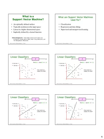
CSCI 5525 Machine Learning Fall 2019 Lecture 6: Support Vector Machine (Part 1) Feb 10 2020 Lecturer: Steven Wu Scribe: Steven Wu We will now derive a different method for linear classification– Support Vector Machine (SVM)– that is based on the idea of margin maximization . 1 Margin Maximization Let us start with an easy case where the data is linearly separable. In this case, there may be infinitely many linear predictors that can achieve zero training error. An intuive solution to break ties is to select the predictor that maximizes the distance between the data points and the decision boundary, which is given by a hyperplane in this case. Now let us write this as an optimization. Figure 1: There are inifinitely many hyperplanes that can classify all the training data correctly. We are looking for the one that maximizes the margin. Image source. For any linear predictor with a weight vector w ∈ R d , the decision boundary is the hyperplane H = { x ∈ R d | w ⊺ x = 0 } . If the linear predictor perfectly classifies has zero training error, then we know that for all ( x i , y i ) ∈ R d × {± 1 } : y i w ⊺ x i > 0 . The distance between the point y i x i and H is given by y i w ⊺ x i � w � 2 The smallest distance from all training points to the hyperplane is given by y i w ⊺ x i min � w � 2 i 1

Then the problem of maximing the margin or distance from the separating hyperplane to the train- ing data is: y i w ⊺ x i max w min � w � 2 i Observe that rescaling the vector w does not actually change the relevant hyperplane and the distances. It suffices to consider the set w ’s such that min i y i w ⊺ x i = 1 . Then the problem of margin maximization becomes 1 max min y i ( w ⊺ x i ) = 1 such that � w � 2 i w Or equivalently, 1 2 � w � 2 min ∀ i, y i ( w ⊺ x i ) ≥ 1 such that (1) 2 w Note that the objectives are the same, but the constraints are different. (Why are two optimiza- tion problems equivalent?) The optimization problem in (1) computes the linear classifier with the largest margin—the support vector machine (SVM) classifier. The solution is also unique. Soft-Margin SVM More generally, the training examples may not be linearly separable. To handle this case, we will introduce slack variables . For each of the n training examples, we will introduce an non-negative variable ξ i , and the optimization problem becomes: n 1 � 2 � w � 2 min 2 + C ξ i such that (2) w i =1 ∀ i, y i ( w ⊺ x i ) ≥ 1 − ξ i (3) ∀ i, ξ i ≥ 0 (4) This is also called the soft-margin SVM. Note that ξ i / � w � 2 is the distance the example i need to move to satisfy the constraint y i ( w ⊺ x i ) ≥ 1 . Equivalently, the soft-margin SVM problem can be written as the following unconstrained optimization problem, which replaces the second term with hinge losses: n 1 � 2 � w � 2 min 2 + C max { 0 , 1 − y i w ⊺ x i } w � �� � i =1 hinge loss We will now introduce a more general method that turns a constrained optimization problem into an unconstrained optimization problem by using the idea of Lagrange duality. 2

Detour of Duality In general, consider the following constrained optimization problem: min w F ( w ) h j ( w ) ≤ 0 ∀ j ∈ [ m ] s.t. For each of the constraint, we can introduce a Lagrangian multiplier λ j ≥ 0 , and write down the following Lagrangian function: m � L ( w , λ ) = F ( w ) + λ j h j ( w ) j =1 Note thats max λ L ( w , λ ) is ∞ whenever the w violates one of the constraints. This means the solution to the following problem min w max L ( w , λ ) λ is exactly the solution to constrained optimization problem. (Why?) Now let’s swap min and max, and consider the following problem: max min w L ( w , λ ) λ Let w ∗ = arg min w (max λ L ( w , λ )) and λ ∗ = arg max λ (min w L ( w , λ )) . We can derive the fol- lowing: max min w L ( w , λ ) = min w L ( w , λ ∗ ) (definition of λ ∗ ) λ ≤ L ( w ∗ , λ ∗ ) (definition of min) ≤ max L ( w ∗ , λ ) (definition of max) λ = min w max L ( w , λ ) (definition of w ∗ ) λ The relationship of maxmin ≤ minmax is called weak duality . Under “mild” condition (e.g. convex quadratic problem, the so-called Slater’s condition), we also have strong duality : max min w L ( w , λ ) = min w max L ( w , λ ) λ λ Under strong duality, we can further write: F ( w ∗ ) = min w max L ( w , λ ) (definition of w ∗ ) λ = max min w L ( w , λ ) (strong duality) λ = min w L ( w , λ ∗ ) (definition of λ ∗ ) ≤ L ( w ∗ , λ ∗ ) (definition of min) � = F ( w ∗ ) + λ ∗ j h j ( w ∗ ) (definition of L ) j 3

Note that since w ∗ is a feasible solution such that h j ( w ∗ ) ≤ 0 for all j , each term λ ∗ j h j ( w ∗ ) ≤ 0 , and so the inequality above should also just be equality. This has the following implications: • (Complementary slackness): last equality implies that λ ∗ j h j ( w ∗ ) = 0 for all j . • (Stationarity): w ∗ is the minimizer of L ( w , λ ∗ ) and thus has gradient zero � ∇ w L ( w ∗ , λ ∗ ) = ∇ F ( w ∗ ) + λ ∗ j ∇ h j ( w ∗ ) = 0 j • (Feasibility): λ j ≥ 0 and h j ( w ∗ ) ≤ 0 for all j . These are also called the KKT conditions, which are necessary conditions for the optimal solutions. But they are sufficient when F is convex and the set of h j are continuously differentiable convex functions. What is KKT? This was previously known as the KT (Kuhn-Tucker) conditions since the cond- tions first appeared in publication by Kuhn and Tucker in 1951. However, later people found out that Karush had stated the conditions in his unpublished master’s thesis of 1939. 4