Lecture 6.1: Quiz 3 prep Use ANOVA Table and formulae to compute F - - PowerPoint PPT Presentation

1

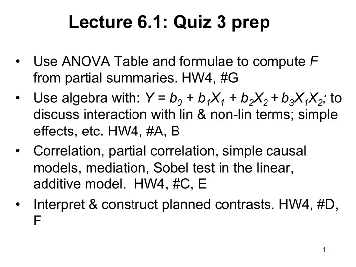
Lecture 6.1: Quiz 3 prep

• Use ANOVA Table and formulae to compute F

from partial summaries. HW4, #G

• Use algebra with: Y = b0 + b1X1 + b2X2 + b3X1X2; to

discuss interaction with lin & non-lin terms; simple effects, etc. HW4, #A, B

• Correlation, partial correlation, simple causal

models, mediation, Sobel test in the linear, additive model. HW4, #C, E

• Interpret & construct planned contrasts. HW4, #D,

F

Q3 Topics; another version

• Topics relevant to Quiz 3 & HW-4
• Partial correl, and its use in testing causal models

with 3 variables. Drawing such causal models, e.g., X è Z è Y.

• Sobel test of mediation
• Design a contrast to test a specific effect; interpret

a given contrast; orthogonal contrasts; t- or F- tests for a contrast

• Linear, X.lin, & quadratic, X.quad, effects of a

quantitative predictor, X; interactions with a categorical predictor, G.

• Compute missing entries in an ANOVA table.

2

HW-4 exercise

• The stress level was measured for each of 24 research
• participants. Six participants were chosen from each of

4 groups: Group 1 was Low in Social Support (e.g., number of friends) and Low in Self-Concept; Group 2 was High in Social Support and Low in Self-Concept; Group 3 was Low in Social Support and High in Self- Concept; and Group 4 was High in Social Support and High in Self-Concept. Shown below are edited sections from a Minitab analysis of the data.

• Complete the ANOVA table; interpret and test (New

question!) a given contrast; calculate the s.e. of a sample mean; describe the effects of Social Support and Self-Concept on stress.

3

• G. DV = stress level; N = 24; n = 6 in each of k = 4 groups.

Group 1 was Low in Social Support and Low in Self- Concept; Group 2 was (Hi, Lo); Group 3 was (Lo, Hi); Group 4 was (Hi, Hi).

Group Mean SocSupp SelfCon l m1 Lo Lo 1 m2 Hi Lo

• 1

m3 Lo Hi

• 1

m4 Hi Hi 1

4

SelfConcept 1 2 All

• SS1 10.4 3.4 6.9

SS2 3.6 3.2 3.4 All 7.0 3.3 5.1

• 1. Complete the 1-way ANOVA table on next slide and

describe the data (using plots and tables, not reg coeffs!).

• 2. Interpret the contrast, l = (m1 - m2) – (m3 - m4), in terms of

SS & SC. Test if l is sig different from 0 (new question!).

Analysis of Variance for Stress Source DF SS MS F P Group aa bb bb bb < bb Error aa 49.80 bb Total aa 272.60

• Pooled StDev = 1.578
• 1. DF: {aa, aa, aa} = { , , }
• 2. SS(Group) =
• 3. MS(Group) =
• ; MS(Error) =
• 4. F =
• 5. P via R or Tables

5

Analysis of Variance for Stress Source DF SS MS F P Group aa bb bb bb < bb Error aa 49.80 bb Total aa 272.60

• Pooled StDev = 1.578
• 1. DF: {aa, aa, aa} = {3, 20, 23}
• 2. SS(Group) =
• 3. MS(Group) =
• ; MS(Error) =
• 4. F =
• 5. P via R or Tables

6

Analysis of Variance for Stress Source DF SS MS F P Group aa bb bb bb < bb Error aa 49.80 bb Total aa 272.60

• Pooled StDev = 1.578
• 1. DF: {aa, aa, aa} = {3, 20, 23}
• 2. SS(Group) = 272.6 – 49.8 = 222.8
• 3. MS(Group) =
• ; MS(Error) =
• 4. F =
• 5. P via R or Tables

7

Analysis of Variance for Stress Source DF SS MS F P Group aa bb bb bb < bb Error aa 49.80 bb Total aa 272.60

• Pooled StDev = 1.578
• 1. DF: {aa, aa, aa} = {3, 20, 23}
• 2. SS(Group) = 272.6 – 49.8 = 222.8
• 3. MS(Group) = 222.8/3 = 74.3
• 4. MS(Error) = 49.8/20 = 2.49;
• 1. s = sqrt(MSE) = sqrt(2.49) = 1.578.
• 5. F = MSB/MSE = 74.3/2.49 = 29.8, p < .00n
• 6. P via R or Tables

8

• Formal test of l = (m1 - m2) – (m3 - m4):

9

l = ai

i

∑

xi, sel

2 = MSw

ai

2

ni

∑

, tN−k = l sel

• r F

1,N−k = tN−k 2

. l = (10.4 − 3.6)− (3.4 − 3.2 = 6.6, se2 = (2.49)* 1 6 + 1 6 + 1 6 + 1 6 ⎛ ⎝ ⎜ ⎞ ⎠ ⎟ = 1.66 t20 = l se = 6.6 1.29 = 5.12; p = 5.2*10−5. The interaction between Soc Support and Self- Concept on the DV is sig; etc. (i.e., describe the interaction using a plot or table).

10

Another HW-4 exercise

• Analysis of SS: SSt = SSb + SSw, etc
• Use ANOVA formulae to compute F

from partial summaries (HW-4)

• I. DV = satisfaction with dispute resolution
• 1. Complete the 1-way ANOVA.
• 2. Ans. What are the relevant quantities, and what formulae

do we have for calculating them?

12

Use of formulae to compute F from partial summaries

• Journal articles sometimes give the means and

s.d.s of k groups without F and p-values. Without the raw data you cannot use software to check the statistics; but you can do it ‘by hand’ using the appropriate formulae.

• Need to calculate: SSb and SSw; the df of these 2

sums of squares; use the df to compute MSb and MSw; compute the F ratio; and test its significance.

13

Tj = xij

i=1 nj

∑

; T = Tj

j=1 k

∑

; N = nj

j=1 k

∑

; C = T 2 / N SStot = xij

2 i

∑

j

∑

− C = SSb + SSw SSj = (nj −1)sj

2, SSw =

SSj

j=1 k

∑

; SSb = (Tj

2 j=1 k

∑

/ nj)− C MSw = SSw /(N − k); MSb = SSb /(k −1) F = MSb / MSw with (k −1, N − k) df.

14

Group nj x j sj

2 Tj = njx j SSj = (nj −1)sj 2

Tj

2 / nj

Manuf 12 25.2 3.6 302.4 39.6 7620.48 Markt 14 32.6 4.8 Resrch 11 28.1 3.6

• ---------------------------------------------- ....

Total 37

• 1067.9

...

C = T2/N = 30821.9, SSw = 155, …, F = 8.53, p < .001.

• Exercise: The manufacturing group is the

'standard' group, and the other two groups are (i) possibly different from the standard, and (ii) possibly different from each other. Set up two

• rthogonal contrasts (involving the group means)

to test these hunches. Carry out the appropriate tests.

• Check that the contrasts l1 = (2, -1, -1) and l2 =

(0, -1, 1) for (man, mar, res), respectively, test the 2 hunches, and are orthogonal.

• For a formal test, we compute the values of l1

and l2, their s.e.’s, and t or F. (Assume the DV = ‘satisfaction’)

15

• Formal test for l1:

16

l = ai

i

∑

xi, sel

2 = MSw

ai

2

ni

∑

, tN−k = l sel

• r F

1,N−k = tN−k 2

. l1 = 2*25.2 −1*32.6 −1*28.1= −10.3, se1

2 = (21.264)* 22

12 + (−1)2 14 + (−1)2 11 ⎛ ⎝ ⎜ ⎞ ⎠ ⎟ = 10.54 t34 = l1 se1 = −10.3 3.247 = −3.172; p = .0032. Satisfaction is sig lower in 'manuf' than the other groups.

• Formal test for l2:

17

l = ai

i

∑

xi, sel

2 = MSw

ai

2

ni

∑

, tN−k = l sel

• r F

1,N−k = tN−k 2

. l2 = 0*25.2 −1*32.6 +1*28.1= −4.5, se2

2 = (21.264)* (−1)2

14 + (1)2 11 ⎛ ⎝ ⎜ ⎞ ⎠ ⎟ = 3.452 t34 = l2 se2 = −4.5 1.858 = −2.422; p = .021. Satisfaction is sig higher in 'marketing' than in 'research'.

HW-4: Interaction between categorical, train, and quantitative, difficulty

• Performance (‘score’) on a task is expected to

depend on the ‘difficulty’ (D, quant: 1, …, 5) of the task, and the level of expertise of the participant (‘train’, T, = novice or expert).

• Can examine linear and quadratic effects of D,

and their interactions with T in a number of ways:

lm(score ~ train * (difficulty + lm(score ~ train * (difficulty + I(difficulty^2)), I(difficulty^2)), or lm(score ~ train * (scale(difficulty) + lm(score ~ train * (scale(difficulty) + I(scale(difficulty)^2)), I(scale(difficulty)^2)), or lm(score ~ train * poly(difficulty, 2)). lm(score ~ train * poly(difficulty, 2)).

18

Describing interactions

• Is there a significant interaction between train and

d.lin, or between train and d.quad? If so, use the plot of means to describe it. (The regression coeffs are usually not reliable by themselves.)

• For some cases, such an informal description is
• sufficient. At other times, we want to be more

precise in our description of the interaction; e.g., does d.lin have a sig effect for novices, or does train have a sig effect when ‘difficulty’ = 3? For this purpose, we need to test formally the specific simple effects.

19

• When there is no interaction, main effects are

easily interpreted. When there is an interaction, main effects can be misleading, and simple effects are more useful for description.

• The preceding 3 models of lm() differ in how

‘difficulty’ or ‘train’ is coded; but they do not differ in substance. How do the models compare in their convenience for testing simple effects?

• The 1st model uses D (> 0) and D2, which are
• correlated. This can lead to the problem of

multicollinearity, namely, ‘large’ s.e’s for the regression coefficients. But sometimes D2 is just the predictor we want!

20

• The other two models yield orthogonal contrasts

for d.lin and d.quad.

• The 3rd model has less code than the 2nd, but is

less transparent. How to visualise the lin and quad components, poly(difficulty, 2)1 and

poly(difficulty, 2)2, of poly(difficulty, 2)?

• scale(difficulty)

scale(difficulty) = (-1.26, -.63, 0, .63, 1.26). It

is standardised with mean = 0, sd = 1, Σai

2 = 4.

• poly(difficulty, 2)1

poly(difficulty, 2)1 = (-.632, -.316, 0, .316, .

632). It has mean = 0 and Σai

2 = 1. It is simply a

rescaling of scale(difficulty)

scale(difficulty).

21

• scale(difficulty)^2

scale(difficulty)^2 = (1.6, .4, 0, .4, 1.6). It is

has mean = 0.8, Σai

2 = 5.44.

• poly(difficulty, 2)2

poly(difficulty, 2)2 = (.535, -.267, -.535, -.

267, .535). It has mean = 0 and Σai

2 = 1. It is

simply a linear transformation of

scale(difficulty)^2 scale(difficulty)^2.

• Not surprisingly, the plot of diff.quad =

scale(difficulty)^2 scale(difficulty)^2 against diff.lin = scale(difficulty) scale(difficulty) looks very similar to that of poly(difficulty, 2)2 poly(difficulty, 2)2 against poly(difficulty, 2)1 poly(difficulty, 2)1 . The ranges of the

variables in the 2 plots are similar and different in predictable ways.

• Also shown is a plot of the data.

22

23

!

When ‘difficulty’ = 3, both diff.lin and diff.quad equal 0. This is a useful property for a regression designed to yield the simple effect of ‘train’ when ‘difficulty’ = 3. Note that poly(difficulty, 2)2

poly(difficulty, 2)2 ≠ 0 when ‘difficulty’

= 3, so the 3rd regression won’t yield the simple effect.

• Note: Unless I am interested in simple effects,

I tend to prefer poly(difficulty, 2)

poly(difficulty, 2) over scale(difficulty) + scale(difficulty) + I(scale(difficulty)^2) I(scale(difficulty)^2) because of its

simplicity.

• Each of the 3 models assumes that the effect
• f ‘difficulty’ is the sum of a linear effect due

to d.lin, and a quadratic effect due to d.quad. The models differ in how they define these 2 effects, but they agree that:

• score ~ train * (d.lin + d.quad), i.e.,

score ~ train * (d.lin + d.quad), i.e.,

• score ~ train + d.lin + d.quad +

score ~ train + d.lin + d.quad + train : d.lin + train : d.quad. train : d.lin + train : d.quad.

24

Examples of main & simple effects

• Main effect of ‘train’. We wish to interpret the

coefficient of ‘train’ in the lm() output as the difference in mean score between ‘experts’ and ‘novices’.

• Simplest to code ‘train’ as (0, 1), and use
• res1 = lm(score ~ train, d)

Coefficients: Estimate Std. Error t value Pr(>|t|) (Intercept) 5.12286 0.31746 16.14 <2e-16 *** trainnovice -0.09429 0.44895 -0.21 0.834

25

• If we want the main effect of ‘train’ from the full

model, we have to code ‘difficulty’ so that both d.lin and d.quad are centered, i.e., have a mean

• f 0. This is achieved with poly(difficulty,

poly(difficulty, 2). 2).

contrasts(d$train) = c(0, 1) res4a = lm(score ~ train * poly(difficulty, 2), d) Coefficients: Estimate Std. Error t value Pr(>|t|) (Intercept) 5.12286 0.24198 21.170 < 2e-16 *** trainnovice -0.09429 0.34222 -0.276 0.78381 poly(D, 2)1 12.82944 2.02458 … … …

Note that the coeff of ‘trainnovice’ is the same as before (-.094).

26

• Simple effect of ‘train’, when ‘difficulty’ = 3.

We wish to interpret the coefficient of ‘train’ in the

lm() output as the difference in mean score

between ‘experts’ and ‘novices’ when ‘difficulty’ = 3. Again code ‘train’ as (0, 1).

• Importantly, code ‘difficulty’ so that so that both

d.lin and d.quad equal 0 when ‘difficulty’ = 3. This is achieved with scale(difficulty).

scale(difficulty).

• res4a = lm(score ~ train * (scale(difficulty)

+ I(scale(difficulty)^2), d)

27

Coefficients: Estimate Std. Error t value Pr(>|t|) (Intercept) 5.9204 0.3771 15.700 < 2e-16 *** train1 -0.9465 0.5333 -1.775 0.08068 . scale(diff) 0.4294 0.2437 1.762 0.08291 . … … … …

• Note that the simple effect of ‘train’, when

‘difficulty’ = 3 is marginally sig (p = .08), whereas the main effect of ‘train’ was not sig (p > .7).

28

• Main effect of ‘difficulty’. We wish to interpret the

coefficients of d.lin and d.quad in the lm() output as the effect of ‘difficulty’ when ‘train’ is ignored.

• Simplest to use
• res1 = lm(score ~ poly(difficulty, 2), d)

Coefficients: Estimate Std. Error t value Pr(>|t|) (Intercept) 5.0757 0.1882 26.976 < 2e-16 *** poly(D, 2)1 8.1980 1.5742 5.208 1.99e-06 *** poly(D, 2)2 -2.6000 1.5742 -1.652 0.103

• The lin, but not the quad, comp is sig.

29

• Simple effect of ‘difficulty’ among novices. We

wish to interpret the coefficients of d.lin and d.quad in the lm() output as the effect of ‘difficulty’ among

• novices. Code ‘train’ = 1 for experts, 0 for novices.

contrasts(d$train) = c(1, 0) res4b = lm(score ~ train * poly(difficulty, 2), d) Coefficients: Estimate Std. Error t value Pr(>|t|) (Intercept) 5.02857 0.24198 20.781 < 2e-16 *** train1 0.09429 0.34222 0.276 0.78381 poly(D,2)1 3.56655 2.02458 1.762 0.08291 . poly(D,2)2 -6.24286 2.02458 -3.084 0.00302 ** tr1:poly(D,2)1 9.26289 2.86319 3.235 0.00193 ** tr1:poly(D,2)2 7.28571 2.86319 2.545 0.01336 *

• Ans: The lin comp is marginal (p = .08); the quad comp is sig

(p = .003)!

30

Classical example: The Yerkes- Dodson Law (1908)

• (Source: Wiki) “The Yerkes–Dodson law is an

empirical relationship between arousal and performance, originally developed by psychologists Robert M. Yerkes and John Dillingham Dodson in 1908.[1] The law dictates that performance increases with physiological or mental arousal, but only up to a

• point. When levels of arousal become too high,

performance decreases. The process is often illustrated graphically as a curvilinear, inverted U- shaped curve which increases and then decreases with higher levels of arousal.”

31

• “Because of task differences, the shape of the

curve can be highly variable.[2] For simple or well-learned tasks, the relationship can be considered linear with improvements in performance as arousal increases. For complex, unfamiliar, or difficult tasks, the relationship between arousal and performance becomes inverse, with declines in performance as arousal increases.”

32

33

Algebraic Appendix, plus a bonus solution for an old HW

34

• score ~ train + d.lin + d.quad +

score ~ train + d.lin + d.quad + train : d.lin + train : d.quad. train : d.lin + train : d.quad.

35

Predictor Coefficient Intercept b0 train2 b1 d.lin b2 d.quad b3 train2:d.lin b4 train2:d.quad b5

• Suppose, when ‘difficulty’ = k, d.lin = 0 = d.quad.

Then score = b0 + b1*train2 describes the simple effect of ‘train’, when ‘difficulty’ = k. To

• btain this simple effect, use I(difficulty - k)

I(difficulty - k)

in lm(). If k = mean(difficulty), can also use

scale(difficulty) in lm().

36

Predictor Coefficient Intercept b0 train2 b1 d.lin b2 d.quad b3 train2:d.lin b4 train2:d.quad b5

• Suppose, when ‘train’ = target, train2 = 0. Then

score = b0 + b2*d.lin + b3*d.quad describes the simple effect of ‘difficulty’ for the target group. To

• btain this simple effect, code ‘train’ so that target

group has train2 = 0.

37

Predictor Coefficient Intercept b0 train2 b1 d.lin b2 d.quad b3 train2:d.lin b4 train2:d.quad b5

Review of the t-test

In a 1-sample t-test, s2 is the estimate of the popn variance, σ2, and s2/n is the estimate of the variance of the sample mean. The s.e. of a statistic is the square root of its variance. Hence,

38

tdf = X − µ est.se(X), where df = df of the estimate of s.e.(X). est.se(X) = s2 / n = s / n, with df = n −1, and tn−1 = X − µ s / n . tdf

2 = F(1, df ), so F can also be used to test H0.

t-tests in Regression

In regression, the statistic of interest is the estimated regression coefficient, bi, and we wish to test if E(bi) = 0. Computer output gives s.e.(bi), as well as t. The df of t is the df of SSresid, and this too is given in the ANOVA table from the regression. In general, the df of SSresid = N – p – 1, where N is the sample size and p is the number of predictors. An example of output with p = 1 follows.

39

tdf = bi est.se(bi), given in output.

40

Coefficients: Estimate Std. Error t value Pr(>|t|) (Intercept) 4.500 0.297 15.151 5.08e-15 *** grpone1 0.300 0.210 1.428 0.164 Residual standard error standard error: 1.627 on 28 degrees of

28 degrees of freedom freedom

Multiple R-squared: 0.06792, Adjusted R-squared: 0.035 F-statistic: 2.04 on 1 and 28 DF 1 and 28 DF, p-value: 0.1642

Note: t2 = 1.4282 = 2.04 = F! 2*(1 - pt(1.428, 28)) = 0.1644, as given above.

t-tests in ANOVA

• Does giving students explicit training on how to
• rganise material (an “organiser”) in a class

improve scores on tests?

• Ss are randomly assigned to one of 3 conditions:

No organiser (‘no.org’), Organiser before lecture (‘pre.org’), and Organiser after lecture (‘post.org’).

• This is a between-S design, and a 1-way ANOVA

is appropriate.

• Analysis of SS: SSt = SSb + SSw,
• F = MSb/MSw, etc

41

42

Data, d, in long form

score group

score group

1 5 no.org 2 4 no.org 3 6 no.org 4 2 no.org 5 2 no.org 6 2 no.org 7 6 no.org 8 4 no.org 9 3 no.org 10 5 no.org 11 4 pre.org 12 5 pre.org 13 3 pre.org … … … 27 6 post.org 28 4 post.org 29 4 post.org 30 7 post.org

# Custom-made function mean.sd = function(x) { c(mean = mean(x, na.rm=T), sd = sd(x, na.rm=T)) } # Data summary by group rs0 = by(d$score, d$group, mean.sd)

43

d$group: no.org mean sd 3.900000 1.595131

• d$group: pre.org

mean sd 4.000000 1.333333

• d$group: post.org

mean sd 5.600000 1.577621 Each of the sd’s, 1.595, 1.33 and 1.578, is an independent estimate of the within-group sd, σ. MSw is the best, pooled est

• f σ2.

To test if mean scores are the same for ‘post.org’ and ‘pre.org’, we would do an indep samples t-test. But what estimate of within-group variance should we use?

• Ans. Better to use MSw than the pooled est from only the

‘post.org’ and ‘pre.org’ groups. The df of the latter is n1 + n2 – 2 = 18; the df of MSw is N – k = 30 – 3 = 27 > 18! (More precise)

44

Analysis of Variance Table Analysis of Variance Table Response: score Df Sum Sq Mean Sq F value Pr(>F) group 2 18.20 9.10 4.0082 0.02991 * Residuals 27 61.30 2.27

Est of var(X1 − X2) = MSw 1 n1 + 1 n2 ⎛ ⎝ ⎜ ⎞ ⎠ ⎟ = MSw 5 = 2.27 5 = .454. Est of se(X1 − X2) = .454 = .674. For 'post.org' vs 'pre.org', t27 = 5.6 − 4.0 .674 = 2.37.

2*(1 - pt(2.37, 27)) = 0.025; so p = .025, 2-tailed.

We haven’t yet considered if this t-test was planned or post-hoc!

45

The 3 group means are: no-org, 3.9; pre-org, 4.0; and post-org, 5.6. rs1 = lm(score ~ group, data=d00)

Coefficients: Estimate Std. Error t value Pr(>|t|) (Intercept) 3.9 3.9000 0.4765 8.185 8.64e-09 *** grouppre.org 0.1 0.1000 0.6739 0.148 0.8831 grouppost.org 1.7 1.7000 0.6739 2.523 0.0178 *

#Default coding is Dummy Coding Dummy Coding print(contrasts(d00$group)) pre.org post.org no.org 0 0 pre.org 1 0 post.org 0 1

46

pre.org post.org no.org 0 0 pre.org 1 0 post.org 0 1

• The implied regression in lm() is:

Y = b0 + b1*pre.org + b2*post.org + e

• Use this eqn. to get the mean score, mj,

for the j’th group, j = 1, 2, 3:

no.org: m1 = b0 + b1*0 + b2*0; b0 = m1 pre.org: m2 = b0 + b1*1 + b2*0; b1 = m2 - m1 post.org: m3 = b0 + b1*0 + b2*1; b2 = m3 - m1

47

• Y = b0 + b1*pre.org + b2*post.org + e

pre.org post.org no.org 0 0 pre.org 1 0 post.org 0 1

• Define Dummy Coding:

– If ‘group’ has k levels, there are k-1 predictors, X1, …, Xk-1 – Designate one level, say, level 1, as the baseline. Each obs in level 1, the control condition, is assigned a value of 0 on all predictors - X1 = 0, …, Xk-1 = 0 – Each obs in level 2 is assigned a value of 1 on X1, and 0 on all

• ther predictors - X1 = 1, X2 = 0, …, Xk-1 = 0

– Each obs in level 3 is assigned a value of 1 on X2, and 0 on all

• ther predictors - X1 = 0, X2 = 1, …, Xk-1 = 0. And so on.

48

Compare output from anova() and summary() rs1 = lm(score ~ group, data=d00) print(anova(rs1)) [slide 8 above]

Analysis of Variance Table Response: score Df Sum Sq Mean Sq F value Pr(>F) group 2 18.20 9.10 4.0082 0.02991 * Residuals 27 61.30 2.27

print(summary(rs1)) [slide 11 above]

Coefficients: Estimate Std. Error t value Pr(>|t|) (Intercept) 3.9000 0.4765 8.185 8.64e-09 *** grouppre.org 0.1000 0.6739 0.148 0.8831 grouppost.org 1.7000 0.6739 2.523 0.0178 *

49

• anova(rs1) gives the familiar omnibus F.

There are no regression coefficients, nor any of the interpretive issues associated with them!

• summary(lm()) yields also a set of

regression coefficients and associated p-

• values. What are the ‘predictor’ variables in

this regression, and what algebraic interpretation do the coefficients have?

• The interpretation of the coeffs depends

critically on how the predictors are defined.

• The coefficients in the regression will often

correspond to the contrasts among group means that we have already discussed.

• The predictors will, in general, not look like

contrasts among means. However, when the contrasts are orthogonal, the predictors are the same as the contrasts (Benoît).

• Note that R calls predictors ‘contrasts’
• What predictors or ‘contrasts’ are used in lm()

as the default? Ans: ‘grouppre.org’ and ‘grouppost.org’.

• How to (a) specify our own ‘contrasts’, and (b)

derive algebraically the interpretation of the coeffs in terms of the group means.

50

51

• The default set of predictors or ‘contrasts’

used in lm() is obtained with contrast.treatment, a particular kind of dummy coding in which level 1 of ‘treatment’ is treated as the baseline or control group (base = 1) . If another level of ‘treatment’, e.g., 2, is the baseline, we would specify base = 2; the predictors or ‘contrasts’ would then be ‘group1’ and ‘group3’.

• With contrast.treatment, the resulting

effects are not really contrasts (the {ai} do not always sum to 0), and they are not

• rthogonal, as will be shown.

52

contrasts(d00$group,2)=contr.treatment(3,base=2, contrasts=TRUE) rs1 = lm(score ~ group, data=d00) print(summary(rs1))

Coefficients: Estimate Std. Error t value Pr(>|t|) (Intercept) 4.0000 0.4765 8.395 5.25e-09 *** group1 -0.1000 0.6739 -0.148 0.8831 group3 1.6000 0.6739 2.374 0.0249 *

• When the contrasts are defined by

‘contr.treatment’, the Intercept Intercept is equal to the mean of the is equal to the mean of the baseline level baseline level - level 1 (3.9) in the 1st analysis, and level 2 (4.0) above.

53

Contrasts

• In a new area of research, we may simply want to

know if a given manipulation (e.g., the grouping variable in a 1-way design) affects the dependent

• variable. The omnibus F-test answers this question.
• However, in many situations, we expect a significant

F and are more interested in specific comparisons among the groups. In this case, we ought to define: – a linear contrast to test each specific comparison, – the contrasts so that they are, if possible, mutually orthogonal.

54

• A contrast is a weighted sum (or average) of

certain group means, where the weights sum to 0. It is a specific explanatory variable (with 1 df) for accounting for differences among the groups.

• If the Group factor has k levels, then Group

has k – 1 df, and there are at most k – 1 non- independent contrasts that can be defined.

• Each contrast can be tested separately for

statistical significance. Defining contrasts so that they are orthogonal (to be defined) assures that the separate tests of the contrasts are approximately independent.

55

In the “organizer’ study, we might be interested in the difference between the pre-organizer and post-organizer population means; the weights, a1 = 0, a2 = 1, a3 = -1, specifies the appropriate contrast: l1 = 0*µ1 + 1*µ2 + (-1)*µ3 = µ2 - µ3

56

• If we are interested in the difference between no
• rganizer and some organizer, the appropriate

weights would be, a1 = 2, a2 = -1, a3 = -1 (or 1, -.5,

• .5):
• l2 = 2*µ1 + (-1)*µ2 + (-1)*µ3 = 2*µ1 - (µ2 + µ3)
• For both contrasts, the {ai} sum to 0.
• Multiplying all {ai} by a constant affects only the

scale or size (and perhaps the sign) of the contrast, not its primary meaning.

• In general, if Level 1 = control, Level 2 = treatment

1, and Level 3 = treatment 2, then the weights (-2, 1, 1) and (0, 1, -1) define, respectively, a contrast

• f ‘treatments’ vs ‘control,’ and a contrast of

‘treat-1’ vs ‘treat-2’. Also, as we shall see, these contrasts are orthogonal.

57

Orthogonal Contrasts

Two contrasts, l1 = ai

i

∑

xi, and l2 = bi

i

∑ xi, are

• rthogonal if the group sample sizes are equal, i.e.,

if ni = n, and if aibi

i

∑

= 0.

(The definition of orthogonality for the case of unequal ni is complicated.) Orthogonal contrasts answer “independent” questions. Knowing if one contrast is significant provides no information about the value of an orthogonal contrast.

“Orthogonal” = “Uncorrelated”

Group X1 X2 1 a1 b1 2 a2 b2 … … … k ak bk

58

Suppose that X1 and X2 are the weights defining 2 contrasts among the k groups. What is the ‘correlation’ between X1 and X2 ? We need the “Sum of Products”, SP, which we wd put in the Numerator of a familiar formula, r = SP/√(SS1SS2). r = 0 iff SP = 0. SP = aibi

i=1 k

∑

− ai

i=1 k

∑

bi

i=1 k

∑

k . Now, if X1 and X2 are true contrasts, ai

i=1 k

∑

= 0 = bi

i=1 k

∑ , and SP =

aibi

i=1 k

∑

. Thus the condition for orthogonality, aibi

i=1 k

∑

= 0, is also the condition for SP = 0, i.e., r = 0.

59

pre.org post.org no.org 0 0 pre.org 1 0 post.org 0 1

• Even though ∑aibi = 0 in dummy coding, ‘pre.org’

and ‘post.org’, are not orthogonal because they are not contrasts; indeed ∑ai = ∑bi = 1 ≠ 0. Intuitively, the 2 effects are correlated, i.e. not

• rthogonal, because they have a common term,

namely, the mean of the baseline group.

• SP = ∑aibi – (∑ai *∑bi )/k = -1/3 ≠ 0; thus the

correlation is not 0.

60

Different sets of orthogonal contrasts when k = 4 groups:

(a) A is quantitative (b) 2 levels of A, 2 levels of B (e.g., 1g. of A, 2 of A, 1 of B, 2 of B). (c) 2x2 factorial (A,B) design (a) (b) (c)

Orthogonal contrasts for a (2x2 + 1) = 5-group design

• The (train, test) groups in the ‘paw-lick’ study are

MM, MS, SM, SS and MM* (where M* = M in a new context). The 1st 4 groups conform to a tidy 2X2 design. Interpret each contrast below!

61

Group lcon ltr lte lT*T 1=MM 1 1 1 1 2=MS 1 1

• 1
• 1

3=SM 1

• 1

1

• 1

4=SS 1

• 1
• 1

1 5=MM* -4

A Paw-Licking Example

Morphine à à Saline Morphine à à Morphine Saline à à Saline Salineà à Morphine Morphine à à Morphine (New Envt) Contrast 1 (new v same) 1 1 1 1

• 4

Contrast 2 Tr: M v S 1 1

• 1
• 1

Contrast 3 Te: M v S Contrast 4 Tr * Te Contrast 5 NA!

(After Siegel, 1975 – See Howell p. 346)

63

• [Students may review this example outside of
• class. Skip the next 5 slides.]
• 1. Five different treatments were tried, one treatment
• n each of 5 different groups of patients who have the

same symptoms. The improvement of each patient was

• measured. Here are the sample size, mean and s.d.,

i.e., (nj, , and sj ) for the 5 groups: (10, 2, .6), (15, 3, .7), (14, 4, .8), (8, 3, .6), and (12, 3, .8). Use a 1-way ANOVA and α = 0.05 to test the null hypothesis that there are no differences in µj among the 5 treatments.

• (Ans. T = 181, N = 59, SSb = 23.7, SSw = 27.98, MSb =

5.925, MSw = 0.518, F = 11.4 with (4, 54) df, so reject H0.)

x j

64

65

66

67

68

Appendix: Possible coding schemes

• What are the predictors or ‘contrasts’ in lm()

when contr.treatment(factor, base=1) is used? Dummy Coding.

• Algebraic interpretation of coeffs in terms of

group means. This depends on the set of ‘contrasts’ used.

• Effect Coding and Orthogonal Coding
• The ‘non-surgical approach’: Multiple, usually

post-hoc, comparisons

• 2-way ANOVA: Between- and Within-S designs.

69

Dummy Coding with a different baseline

• contrasts(d00$group,2) =

contr.treatment(3, base base=2, contrasts=TRUE)

$group 1 3 no.org 1 0 pre.org 0 0 post.org 0 1

• Check that lm() gives: Intercept = mean for

level 2 (4.0), and the other 2 coeffs are b1 = m2 - m1 and b2 = m2 - m3 .

70

rs1 = lm(score ~ group, data=d00) print(summary(rs1))

Coefficients: Estimate Std. Error t value Pr(>|t|) (Intercept) 4.0000 0.4765 8.395 5.25e-09 *** group1 -0.1000 0.6739 -0.148 0.8831 group3 1.6000 0.6739 2.374 0.0249 *

• The p-values are different because the

predictors are different. E.g., ‘group3’ is the mean difference between level 2, the new baseline, and level 3.

71

• In dummy coding, obs in the baseline group

are assigned 0 on all k-1 predictors. Suppose we instead assigned these obs a value of -1 on all k-1 predictors. This would be called Effect

• Coding. We offer an algebraic rationale.

effect1 effect2 no.org -1 -1 pre.org 1 0 post.org 0 1

• The implied regression in lm() is:

Y = c0 + c1*effect1 + c2*effect2 + e

Effect Coding

72

effect1 effect2 no.org -1 -1 pre.org 1 0 post.org 0 1

• The implied regression in lm() is:

Y = c0 + c1*effect1 + c2*effect2 + e

• Use this eqn. to get the mean score, mj, for

the j’th group, j = 1, 2, 3:

• no.org: m1 = c0 + c1*(-1) + c2*(-1) = c0 - c1 - c2
• pre.org: m2 = c0 + c1*1 + c2*0 = c0 + c1
• post.org: m3 = c0 + c1*0 + c2*1 = c0 + c2
• Adding these 3 eqns: c0 = (m1+m2+m3)/3 =
• So c1 = m2 - , and c2 = m3 - .

m m m

73

• With Effect Coding

– The intercept equals the unweighted grand mean – The coefficients index the difference between the associated group mean and the grand mean; i.e., it indexes the ‘effect’ of being in that group (relative to the grand mean) – The p-values for the coeffs will be different from those obtained with dummy coding

• The 2 effects are not orthogonal because they

have a common term, the grand mean.

• Our choice of coding scheme (e.g., dummy vs.

effect vs. orthogonal coding; choice of control group) depends on what we want to test. We now know how to use (i) R to specify the ‘contrasts’ we want; and (ii) Algebra to interpret the coeffs.

74

d00$gpeffect = d00$group contrasts(d00$gpeffect,2) = cbind(effect1=c(-1,1,0), effect2=c(-1,0,1)) rs2a = lm(score ~ gpeffect, data=d00) print(summary(rs2a)) print(rs2a$contrasts)

Coefficients: Estimate Std. Error t value Pr(>|t|) (Intercept) 4.5000 0.2751 16.358 1.55e-15 *** gpeffecteffect1 -0.5000 0.3890 -1.285 0.20964 gpeffecteffect2 1.1000 0.3890 2.827 0.00873 **

75

• Orthogonal Coding

d00$gportho = d00$group contrasts(d00$gportho,2) = cbind(some.org=c(-2,1,1), pre.post=c(0,-1,1)) rs2b = lm(score ~ gportho, data=d00) print(summary(rs2b)) print(rs2b$contrasts)

Coefficients: Estimate Std. Error t value Pr(>|t|) (Intercept) 4.5000 0.2751 16.358 1.55e-15 *** gporthosome.org 0.3000 0.1945 1.542 0.1347 gporthopre.post 0.8000 0.3369 2.374 0.0249 *

Residual standard error: 1.507 on 27 degrees of freedom Multiple R-squared: 0.2289, Adjusted R-squared: 0.1718 F-statistic: 4.008 on 2 and 27 DF

2 and 27 DF, p-value: 0.02991

76

Orthogonal contrasts

Level ‘1’ is ‘control’; ‘2’,‘3’ are treatmts Levels are quantitative l1 l2 a*b llin lquad a*b 1 2 1 1 1 2

• 1

1

• 1
• 2

3

• 1
• 1

1

• 1

1

• 1

SUM

77

• Sometimes we want to test only 1, not both,
• contrasts. Use C()

contr1 = as.matrix(c(-2,1,1), ncol=1) d00$grpone = C(d00$group,contr1,1) rs3 = lm(score ~ grpone, data=d00) print(summary(rs3)) [Note change in df, and change in p-value for ‘grpone1’ coeff!]

Coefficients: Estimate Std. Error t value Pr(>|t|) (Intercept) 4.500 0.297 15.151 5.08e-15 *** grpone1 0.300 0.210 1.428 0.164 Residual standard error: 1.627 on 28 degrees of freedom Multiple R-squared: 0.06792, Adjusted R-squared: 0.03464 F-statistic: 2.04 on 1 and 28 DF

1 and 28 DF, p-value: 0.1642