Lecture 4.2: Quiz 2 prep; HW Solutions; Probability Theory Topics - PowerPoint PPT Presentation
Lecture 4.2: Quiz 2 prep; HW Solutions; Probability Theory Topics for Quiz 2 , Fri 10/24: HW-3, especially # B, H, J, K, L, M HW-2, especially # 8-10, 13 HW-1 (except # 9) Old Topics (content) t-tests, 2 tests;
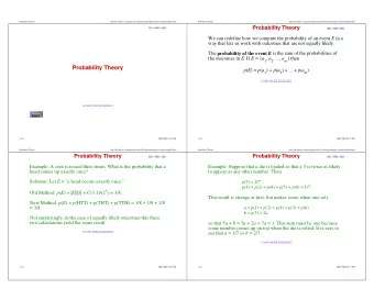
Lecture 4.2: Quiz 2 prep; HW Solutions; Probability Theory • Topics for Quiz 2 , Fri 10/24: • HW-3, especially # B, H, J, K, L, M • HW-2, especially # 8-10, 13 • HW-1 (except # 9) • ‘Old’ Topics (content) – t-tests, χ 2 tests; Confidence Intervals for µ, p, and σ 2 ; Power; Simple Regression; CLT – lm() output to examine Interaction, poly(X, 2) – Calculate µ and σ 2 for discrete distrn – Simple calculations of Probability; P(1 < χ 3 2 < 6.25). 1
New Topics for Quiz 2 • Conditional Probability • Examples, Axioms and Laws of Probability Theory • ‘By hand’ calculations in Regression • More on linear vs non-linear effects, and interaction • Examples of prob calculations. (Already can solve “sample size reqd for margin of error to be 5%”, “budget required so that P(solvency) = 95%”) • Homogeneity of variance – test and transformations that remedy heterogeneity 2
Psy 10/Stat 60: Quiz 7, 2006 Students use the course material (lectures, stat text, own notes, problems and solutions, etc.) to varying degrees, and level of use defines “ an inverse index of a student’s ‘preparedness’ , X , on a 0-10 scale: “ X = 0” means “highly prepared”, … , and “ X = 10” means “unprepared.” Y measures a student’s statistical sophistication one year after the course, 0 ≤ Y ≤ 10. It may be assumed that a relationship between X and Y , if one exists, would be approximately linear. The ( x i , y i ) values for a random sample of 30 students were obtained, and a partial summary of the data follows. 3
Ans : We must first use these quantities to calculate the 5 or so statistics needed for correlation & regression: 4
5
3. Calculate the correlation coefficient, r , between X and Y . Test whether the observed r is statistically significant, stating your significance level , α , and your alternative hypothesis . (50) 4. State briefly your reasoning for your choice of alternative hypothesis in #3 above. (20) 5. Calculate the proportion of variance in Y that is explained by X . [ Ans . Prop explained variance = r 2 = 17.1%.] 6. Calculate the regression equation of Y on X . [ Ans . b = -.529, a = 8.17, so regression eqn is: y = 8.17 – 0.529 x ] 7. What do you conclude about the relation between the variables in this study? 6
Example (HW-3, #M) : The cost, X , of treating a patient varies with the type and seriousness of the medical problem, and with other factors. X is coded as $100, $300, $500, or $700, and its probability distribution is: ∑ µ ≡ E ( X ) = x i = 3.2; p i i σ 2 ≡ E [( X − µ ) 2 ] = E ( X 2 ) − µ 2 = 13.8 − 3.2 2 = 3.56. σ = 1.89. 7
µ T = 16 i µ = 16 i 3.2 = 51.2, 2 = 16 i σ 2 = 16 i 3.56 = 56.96; σ T = 7.55. σ T 8
Probability as Area under the Curve 9
Joint prob : P(‘X < b’ AND ‘X > a’) = P(‘a < X < b’) 10
Examples > pnorm(1.645) [1] 0.950015 > pnorm(1.645, lower = F) [1] 0.04998491 > qnorm(.05) [1] -1.644854 > qnorm(.05, lower = F) [1] 1.644854 > pt(2.2, 8, lower = F) [1] 0.02949695 > pchisq(3.84, 1, lower = F) [1] 0.050043 11
Conditional Probability • Suppose we know the distrn of the scores, X, of 100 persons. E.g., 80 have X > 10; 50 have X > 15; 20 have X > 19, etc. • What proportion have X > 15? Ans. .5 • Among those with X > 10 , what proportion have X > 15? This is the conditional prob , P(X > 15 | X > 10). Ans. 50/80 = .625 (not .5!) 12
Conditional Probability 13
P( Q > x ) .95 .80 .70 .50 .30 .20 .05 .02 x 1.2 2.3 3.0 4.4 6.1 7.3 11.1 13.4 • (Psy 10/Stat 60, Quiz 2) A careful assessment of the quality (Q) of a large pool of applicants for a certain type of job gives the following distribution of quality . For a given level, x , of quality , we show the proportion, Prob( Q > x ), of applicants with quality greater than x . 14
P( Q > x ) .95 .80 .70 .50 .30 .20 .05 .02 x 1.2 2.3 3.0 4.4 6.1 7.3 11.1 13.4 • Calculate Prob(4.4 < Q < 7.3). (20) (Ans. .5 - .2 = .3.) • Only applicants with Q values of 2.3 or more are invited for an interview. Among interviewees (i) what is the conditional probability that the quality of an interviewee would be greater than 4.4? (30) (ii) what is the conditional probability that the quality of an interviewee would be less than 15 6.1? (30)
Answers (i) P(Q > 4.4 | Q > 2.3) = P(Q > 4.4 and Q > 2.3)/P(Q > 2.3) = P(Q > 4.4)/P(Q > 2.3) = .5/.8 = .625 . (ii) P(Q < 6.1 | Q > 2.3) = P(Q < 6.1 and Q > 2.3)/P(Q > 2.3) = P(2.3 < Q < 6.1)/P(Q > 2.3) = (.8 - .3)/(.8) = .5/.8 = .625 . 16
Probability and Causal Reasoning • In a recent (10/9/09) article, since retracted: – 4% of healthy persons carry the virus, XMRV – 66 out of 101 chronic fatigue syndrome patients carry XMRV – Maybe XMRV is a ‘ passenger virus ’ : CFS è XMRV – Maybe Cause0 causes people to get CFS and XMRV – Or maybe XMRV causes CFS: XMRV è CFS • The statistics here is trivial. Under the null, 1 – pbinom(65, 101, .04) = 0! • It ’ s the causal story that ’ s complex. The initial reports (2006) were followed by a large number of studies in which no association was found between XMRV and cancer or CFS. It has not been established [in 2013] that XMRV can infect humans, nor has it been demonstrated that XMRV is associated with or causes human 17 disease.
Motivation for studying PT • Probability Theory (PT) is inherently interesting; but it also has instrumental value! • PT provides theory underlying Stats and Psych: (a) ‘large’ or ‘extreme’ deviation = deviation with a ‘low ’ ! probability (basis for Statistical Inference) (b) Mean (i.e., Expected Value), median, mode; variance, etc. are probabilistic concepts (c) Laws of Large Numbers; Central Limit Theorem (d) ‘best’ estimate of a parameter (e.g., µ ) is the value that makes the observed data most probable or likely (the Maximum Likelihood principle) (e) ‘Law of small numbers’ – Kahneman & Tversky • But not every concept is probabilistic! E.g., ‘least squares’ 18
The CLT per Wiki Tijms (2004, p. 169) writes: The central limit theorem has an interesting history. The first version of this theorem was postulated by the French-born mathematician Abraham de Moivre who, in a remarkable article published in 1733, used the normal distribution to approximate the distribution of the number of heads resulting from many tosses of a fair coin. This finding was far ahead of its time, and was nearly forgotten until the famous French mathematician Pierre-Simon Laplace rescued it from obscurity in his monumental work Théorie Analytique des Probabilités , which was published in 1812. Laplace expanded De Moivre's finding … It was not until the nineteenth century was at an end that the importance of the central limit theorem was discerned, when, in 1901, Russian mathematician Aleksandr Lyapunov defined it in general terms and proved precisely how it worked mathematically. Nowadays, the central limit theorem is considered to be the unofficial sovereign of probability theory . 19
Sir Francis Galton ( Natural Inheritance , 1889) described the Central Limit Theorem as: I know of scarcely anything so apt to impress the imagination as the wonderful form of cosmic order expressed by the "Law of Frequency of Error". The law would have been personified by the Greeks and deified, if they had known of it. It reigns with serenity and in complete self-effacement, amidst the wildest confusion. The huger the mob, and the greater the apparent anarchy, the more perfect is its sway. It is the supreme law of Unreason. Whenever a large sample of chaotic elements are taken in hand and marshaled in the order of their magnitude, an unsuspected and most beautiful form of regularity proves to have been latent all along. 20
Technical Note • The proof of the CLT relies, in turn, on various limits involving the logarithm and exponential functions, such as: • As n -> ∞ , [1 + (a/n)] n -> e a . • For small x , log (1 + x) ≈ x, or, equivalently, • For small x , e x ≈ 1 + x. • The ‘ x ’ in these approximations refers to 1/n , n large, in the proof of the CLT. The CLT is an example of ‘large sample’ theory. 21
Least Squares : An algebraic, not probabilistic, principle for choosing ‘best’ estimates of parameters. We used it in regression estimation earlier. Ex : x 1 , x 2 , … , x n are independent obs from a population with mean, µ . What is ‘best’ est, m , of µ . For each x i , define ‘error’ or ‘loss’ as ( x i - m ) 2 . What value of m minimizes (makes ‘ least ’ ) the sum of squared errors, ∑ ( x i - m ) 2 ? x Recall the definition of the mean, , and note that the Sum of Squares, SS = ∑ ( x i - ) 2 , does not x depend on m . 22
• Then, we wish to minimize ∑ ∑ C ≡ ( x i − m ) 2 = − x ) + ( x − m )] 2 [( x i ∑ ∑ ∑ = ( x i − x ) 2 + 2 ( x i − x ) ( x − m ) + ( x − m ) 2 ∑ = SS + 2( x − m ) ( x i − x ) + n ( x − m ) 2 = SS + 0 + n ( x − m ) 2 , which is a min when m = x . • This shows that the sample mean has the useful, ‘ least squares ’ property 23
Recommend
More recommend
Explore More Topics
Stay informed with curated content and fresh updates.
