Lecture 24: Perceptrons Regression Prof. Julia Hockenmaier - PowerPoint PPT Presentation
CS440/ECE448: Intro to Artificial Intelligence Lecture 24: Perceptrons Regression Prof. Julia Hockenmaier juliahmr@illinois.edu http://cs.illinois.edu/fa11/cs440 Linear regression Squared Loss Given
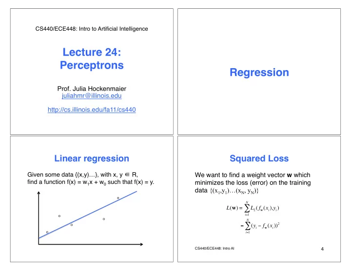
CS440/ECE448: Intro to Artificial Intelligence � Lecture 24: Perceptrons � Regression � Prof. Julia Hockenmaier � juliahmr@illinois.edu � � http://cs.illinois.edu/fa11/cs440 � � � Linear regression � Squared Loss � Given some data {(x,y)…}, with x, y ∈ R, � We want to find a weight vector w which find a function f(x) = w 1 x + w 0 such that f(x) = y. � minimizes the loss (error) on the training data {(x 1 ,y 1 )…(x N , y N )} o N ! L ( w ) = L 2 ( f w ( x i ), y i ) i = 1 o o N ! ) 2 o = ( y i " f w ( x i ) o i = 1 CS440/ECE448: Intro AI � 4 �
Linear regression � Gradient descent � We need to minimize the loss on the training In general, we won ʼ t be able to find a closed- data: w = argmin w Loss(f w ) form solution, so we need an iterative (local � search) algorithm. � We need to set partial derivatives of Loss(f w ) � � with respect to w1, w0 to zero. � We will start with an initial weight vector w, � and update each element iteratively in the This has a closed-form solution for linear direction of its gradient: � w i := w i – ! d/dw i Loss( w ) regression (see book). � CS440/ECE448: Intro AI � 6 � Binary classification Binary classification � with Naïve Bayes � For each item x = (x 1…. x d ) , we compute � The input x = (x 1…. x d ) ∈ R d is real-valued vector, � f k ( x ) = P( x | C k )P(C k ) = P(C k ) " i P(x i |C k ) We want to learn f( x) . for both class C 1 and C 2 � � + + + + � + + x x f( x ) = 0 + + x 2 + + We assign class C 1 to x if f 1 ( x ) > f 2 ( x ) + + + + x x + + x x x x Equivalently, we can define a ʻ discriminant function ʼ x x x x We assume the f( x ) = f 1 ( x ) - f 2 ( x ) x x x x + + two classes are x x and assign class C 1 to x if f( x ) > 0 x x linearly separable � x 1 CS440/ECE448: Intro AI � 7 � CS440/ECE448: Intro AI � 8 �
Binary classification � Binary classification � The weight vector w defines the orientation of the decision boundary. � The input x = (x 1…. x d ) ∈ R d is real-valued vector � The bias term w 0 defines the perpendicular We want to learn f( x) . distance of the decision boundary to the origin. � � We assume the classes are linearly separable, so � + � + � + � we choose a linear discrimant function: x 2 + � x � + � + � ! w 0 f( x) = w � x + w 0 + � + � w x � + � – w = (w 1…. w d ) ∈ R d is a weight vector � x � – w 0 is a bias term � x � x � x � – -w 0 is also called a threshold: - w 0 = w � x x � x � x � x � w x 1 CS440/ECE448: Intro AI � 10 � Binary classification � Binary classification � Equivalently, redefine Our classification hypothesis then becomes � x = (1, x 1…. x d ) ∈ R d+1 h w ( x ) = 1 if f( x ) = w � x # 0 w = (w 0, w 1…. w d ) ∈ R d+1 � 0 otherwise f( x) = w � x � Define C 1 = 1 C 2 = 0 � We can also think of h w (x) as a threshold function. � � h w ( x ) = Threshold( w � x ), Our classification hypothesis then becomes � h w (x) = 1 if f( x ) = w � x # 0 where Threshold( z ) = 1 if z # 0 0 otherwise 0 otherwise � � �
Learning the weights � Observations � If we classify an item ( x, y) correctly, We need to choose w to minimize we don ʼ t need to change w. classification loss. � � If we classify an item ( x, y) incorrectly, But we cannot compute this in closed form, � there are two cases: � because the gradient of w is either 0 or undefined. � – y = 1 ( above the true decision boundary) h w ( x) = 0 ( below the true decision boundary) � We need to move our decision boundary up! Iterative solution: � � – Start with initial weight vector w. � – y = 0 ( below the true decision boundary) h w ( x) = 1 ( above the true decision boundary) – For each example ( x, y) update weights w until all items We need to move our decision boundary down! are correctly classified. � CS440/ECE448: Intro AI � 13 � CS440/ECE448: Intro AI � 14 � Learning the weights Learning the weights � (initial attempt) � Evaluating y - h w ( x ) will tell us what to do: Iterative solution: � – h w ( x ) is correct: y - h w ( x ) = 0 (stay!) – Start with initial weight vector w. � – For each example ( x, y) update weights w until all items – If y = 1 , but we predict h w ( x ) = 0 are correctly classified. y - h w ( x) = 1 – 0 = 1 � (move up!) Update rule: � For each example ( x, y) update each weight w i : � – If y = 0 , but we predict h w ( x ) = 1 w i := w i + (y - h w ( x ))x i y - h w ( x) = 0 – 1 = – 1 � (move down!) CS440/ECE448: Intro AI � 15 � CS440/ECE448: Intro AI � 16 �
There is a problem: � Learning the weights � Real data is not perfectly separable. � Observation: � There will be noise, and our features may not be sufficient. � When we ʼ ve only seen a few examples, we want the weights to change a lot. � + + + + � + + x x f( x ) = 0 + + x 2 + + After we ʼ ve seen a lot of examples, we want the + + + + x x weights to change less and less, because we can + + x x x x now classify most examples correctly. � x x x x � x x x x + + x x x x Solution: We need a learning rate which decays over time. � x 1 CS440/ECE448: Intro AI � 17 � CS440/ECE448: Intro AI � 18 � Batch/Epoch Learning the weights Perceptron Learning (Perceptron algorithm) � � � Choose a convergence criterion (#epochs, min | ! w |, …) � Iterative solution: � Choose a learning rate " , an initial w � – Start with initial weight vector w. � Repeat until convergence: � – For each example ( x, y) update weights w until w has � ! w = # x " err x � (sum over training set holding w ) � converged (does not change significantly anymore) � w $ w + ! w (update with accumulated changes) � � � Perceptron update rule ( ʻ online ʼ ): � – For each example ( x, y) update each weight w i : Now it always converges, regardless of " (will influence w i := w i + ! (y - h w ( x ))x i the rate), and whether or not training points are linearly � – ! decays over time t (t=#examples) e.g ! = n/(n+t) CS440/ECE448: Intro AI � 19 � 20 �
Recommend
More recommend
Explore More Topics
Stay informed with curated content and fresh updates.
