Machine Learning (CSE 446): PCA (continued) and Learning as - PowerPoint PPT Presentation

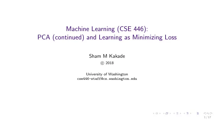
Machine Learning (CSE 446): PCA (continued) and Learning as Minimizing Loss Sham M Kakade � 2018 c University of Washington cse446-staff@cs.washington.edu 1 / 17

PCA: continuing on... 1 / 17

Dimension of Greatest Variance Assume that the data are centered , i.e., that � � � x n � N mean = 0 . n =1 1 / 17

Dimension of Greatest Variance Assume that the data are centered , i.e., that � � � x n � N mean = 0 . n =1 1 / 17

Projection into One Dimension Let u be the dimension of greatest variance, where � u � 2 = 1 . p n = x n · u is the projection of the n th example onto u . Since the mean of the data is 0 , the mean of � p 1 , . . . , p N � is also 0 . N � This implies that the variance of � p 1 , . . . , p N � is 1 p 2 n . N n =1 The u that gives the greatest variance, then, is: N � ( x n · u ) 2 argmax u n =1 2 / 17

Finding the Maximum-Variance Direction N � ( x n · u ) 2 argmax u n =1 s.t. � u � 2 = 1 (Why do we constrain u to have length 1?)   x ⊤ 1   x ⊤   � Xu � 2 , s.t. � u � 2 = 1 . If we let X =  , then we want: argmax   . .  . u x ⊤ N 2- This is PCA in one dimension! 3 / 17

Linear algebra review: things to understand ◮ � x � 2 is the Euclidean norm. ◮ What is the dimension of Xu ? ◮ What is i -th component of Xu ? ◮ Also, note: � u � 2 = u ⊤ u ◮ So what is � Xu � 2 ? 4 / 17

Constrained Optimization The blue lines represent contours : all points on a blue line have the same objective function value. 5 / 17

Deriving the Solution Don’t panic. � Xu � 2 , s.t. � u � 2 = 1 argmax u ◮ The Lagrangian encoding of the problem moves the constraint into the objective: λ � Xu � 2 − λ ( � u � 2 − 1) � Xu � 2 − λ ( � u � 2 − 1) max min ⇒ min λ max u u 6 / 17

Deriving the Solution Don’t panic. � Xu � 2 , s.t. � u � 2 = 1 argmax u ◮ The Lagrangian encoding of the problem moves the constraint into the objective: λ � Xu � 2 − λ ( � u � 2 − 1) � Xu � 2 − λ ( � u � 2 − 1) max min ⇒ min λ max u u ◮ Gradient (first derivatives with respect to u ): 2 X ⊤ Xu − 2 λ u ◮ Setting equal to 0 leads to: λ u = X ⊤ Xu ◮ You may recognize this as the definition of an eigenvector ( u ) and eigenvalue ( λ ) for the matrix X ⊤ X . ◮ We take the first (largest) eigenvalue. 6 / 17

Deriving the Solution: Scratch space 7 / 17

Deriving the Solution: Scratch space 7 / 17

Deriving the Solution: Scratch space 7 / 17

Variance in Multiple Dimensions So far, we’ve projected each x n into one dimension. To get a second direction v , we solve the same problem again, but this time with another constraint: � Xv � 2 , s.t. � v � 2 = 1 and u · v = 0 argmax v (That is, we want a dimension that’s orthogonal to the u that we found earlier.) Following the same steps we had for u , the solution will be the second eigenvector. 8 / 17

“Eigenfaces” Fig. from https://github.com/AlexOuyang/RealTimeFaceRecognition 9 / 17

Principal Components Analysis ◮ Input: unlabeled data X = [ x 1 | x 2 | · · · | x N ] ⊤ ; dimensionality K < d ◮ Output: K -dimensional “subspace”. ◮ Algorithm: 1. Compute the mean µ 2. compute the covariance matrix : � Σ = 1 ( x i − µ )( x i − µ ) ⊤ N i 3. let � λ 1 , . . . , λ K � be the top K eigenvalues of Σ and � u 1 , . . . , u K � be the corresponding eigenvectors ◮ Let � U = [ u 1 | u | · · · | u K ] Return � U You can read about many algorithms for finding eigendecompositions of a matrix. 10 / 17

Alternate View of PCA: Minimizing Reconstruction Error Assume that the data are centered . Find a line which minimizes the squared reconstruction error. 11 / 17

Alternate View of PCA: Minimizing Reconstruction Error Assume that the data are centered . Find a line which minimizes the squared reconstruction error. 11 / 17

Projection and Reconstruction: the one dimensional case ◮ Take out mean µ : ◮ Find the “top” eigenvector u of the covariance matrix. ◮ What are your projections? ◮ What are your reconstructions, � x N ] ⊤ ? X = [ � x 1 | � x 2 | · · · | � ◮ Whis is your reconstruction error? � 1 x i ) 2 =?? ( x i − � N i 12 / 17

Alternate View: Minimizing Reconstruction Error with K -dim subspace. Equivalent (“dual”) formulation of PCA: find an “orthonormal basis” u 1 , u 2 , . . . u K which minimizes the total reconstruction error on the data: � 1 ( x i − Proj u 1 ,... u K ( x i )) 2 argmin N orthonormal basis: u 1 , u 2 ,... u K i Recall the projection of x onto K -orthonormal basis is: K � Proj u 1 ,... u K ( x ) = ( u i · x ) u i j =1 The SVD “simultaneously” finds all u 1 , u 2 , . . . u K 13 / 17

Choosing K (Hyperparameter Tuning) How do you select K for PCA? Read CIML (similar methods for K -means) 13 / 17

PCA and Clustering There’s a unified view of both PCA and clustering. ◮ K -Means chooses cluster-means so that squared distances to data are small. ◮ PCA chooses a basis so that reconstruction error of data is small. Both attempt to find a “simple” way to summarize the data: fewer points or fewer dimensions. Both could be used to create new features for supervised learning 14 / 17

Loss functions 14 / 17

Perceptron A model and an algorithm, rolled into one. Model: f ( x ) = sign ( w · x + b ) , known as linear , visualized by a (hopefully) separating hyperplane in feature-space. Algorithm: PerceptronTrain , an error-driven, iterative updating algorithm. 15 / 17

A Different View of PerceptronTrain : Optimization “Minimize training-set error rate”: loss N � 1 min � y n · ( w · x + b ) ≤ 0 � N w ,b n =1 � �� � ǫ train ≡ zero-one loss margin = y · ( w · x + b ) 16 / 17

A Different View of PerceptronTrain : Optimization “Minimize training-set error rate”: loss � N 1 min � y n · ( w · x + b ) ≤ 0 � N w ,b n =1 � �� � ǫ train ≡ zero-one loss margin = y · ( w · x + b ) This problem is NP-hard; even solving trying to get a (multiplicaive) approximatation is NP-hard. 16 / 17

A Different View of PerceptronTrain : Optimization loss “Minimize training-set error rate”: N � 1 min � y n · ( w · x + b ) ≤ 0 � N margin = y · ( w · x + b ) w ,b n =1 � �� � ǫ train ≡ zero-one loss What the perceptron does: loss � N 1 min max( − y n · ( w · x + b ) , 0) N � �� � w ,b n =1 perceptron loss margin = y · ( w · x + b ) 16 / 17

A Different View of PerceptronTrain : Optimization “Minimize training-set error rate”: N � 1 min � y n · ( w · x + b ) ≤ 0 � N w ,b n =1 � �� � ǫ train ≡ zero-one loss What the perceptron does: � N 1 min max( − y n · ( w · x + b ) , 0) � �� � N w ,b n =1 perceptron loss 16 / 17

A Different View of PerceptronTrain : Optimization “Minimize training-set error rate”: N � 1 min � y n · ( w · x + b ) ≤ 0 � N w ,b n =1 � �� � ǫ train ≡ zero-one loss What the perceptron does: N � 1 min max( − y n · ( w · x + b ) , 0) � �� � N w ,b n =1 perceptron loss 16 / 17

Smooth out the Loss? 17 / 17