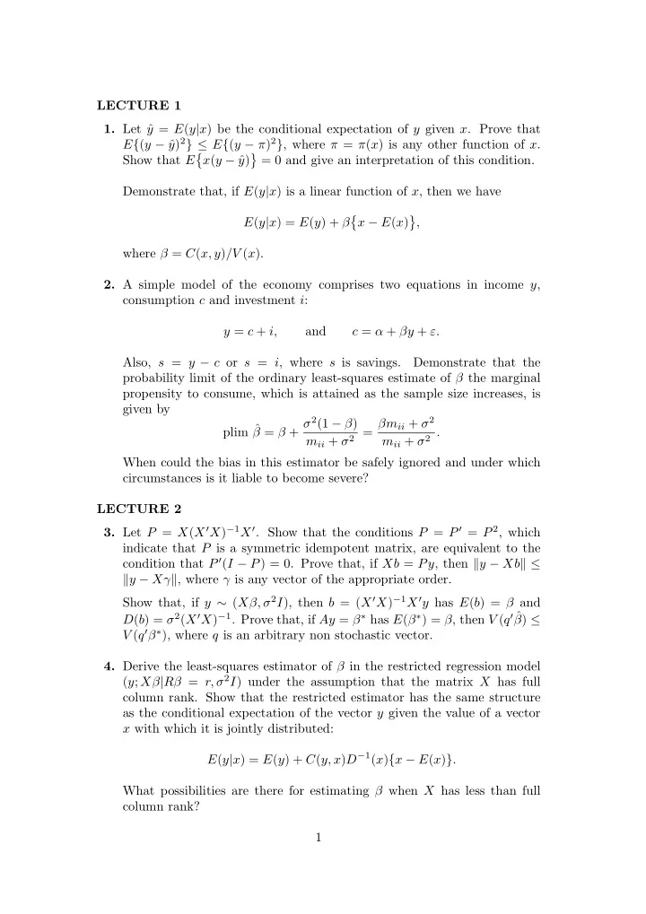
LECTURE 1 1. Let y = E ( y | x ) be the conditional expectation of y - PDF document

LECTURE 1 1. Let ˆ y = E ( y | x ) be the conditional expectation of y given x . Prove that y ) 2 } ≤ E { ( y − π ) 2 } , where π = π ( x ) is any other function of x . E { ( y − ˆ � � Show that E x ( y − ˆ y ) = 0 and give an interpretation of this condition. Demonstrate that, if E ( y | x ) is a linear function of x , then we have � � E ( y | x ) = E ( y ) + β x − E ( x ) , where β = C ( x, y ) /V ( x ). 2. A simple model of the economy comprises two equations in income y , consumption c and investment i : y = c + i, and c = α + βy + ε. Also, s = y − c or s = i , where s is savings. Demonstrate that the probability limit of the ordinary least-squares estimate of β the marginal propensity to consume, which is attained as the sample size increases, is given by β = β + σ 2 (1 − β ) m ii + σ 2 = βm ii + σ 2 plim ˆ m ii + σ 2 . When could the bias in this estimator be safely ignored and under which circumstances is it liable to become severe? LECTURE 2 3. Let P = X ( X ′ X ) − 1 X ′ . Show that the conditions P = P ′ = P 2 , which indicate that P is a symmetric idempotent matrix, are equivalent to the condition that P ′ ( I − P ) = 0. Prove that, if Xb = Py , then � y − Xb � ≤ � y − Xγ � , where γ is any vector of the appropriate order. Show that, if y ∼ ( Xβ, σ 2 I ), then b = ( X ′ X ) − 1 X ′ y has E ( b ) = β and D ( b ) = σ 2 ( X ′ X ) − 1 . Prove that, if Ay = β ∗ has E ( β ∗ ) = β , then V ( q ′ ˆ β ) ≤ V ( q ′ β ∗ ), where q is an arbitrary non stochastic vector. 4. Derive the least-squares estimator of β in the restricted regression model ( y ; Xβ | Rβ = r, σ 2 I ) under the assumption that the matrix X has full column rank. Show that the restricted estimator has the same structure as the conditional expectation of the vector y given the value of a vector x with which it is jointly distributed: E ( y | x ) = E ( y ) + C ( y, x ) D − 1 ( x ) { x − E ( x ) } . What possibilities are there for estimating β when X has less than full column rank? 1

5. Find expressions for the ordinary least-squares estimators b 1 , b 2 of β 1 , β 2 in the partitioned regression model ( y ; X 1 β 1 + X 2 β 2 , σ 2 I ). Find simplified forms for these estimators in the case where the columns of X 1 are orthogonal to those of X 2 , and show that, if all of the columns of X = [ X 1 , X 2 ] are mutually orthogonal, then the k regression parameters 2 ] ′ can be estimated via k univariate ordinary least-squares in β = [ β ′ 1 , β ′ regressions. What do you understand by the omitted variables bias? LECTURE 3 6. Derive the so-called Yule–Walker equations      σ 2  γ 0 γ 1 γ 2 α 0 ε  =  , γ 1 γ 0 γ 1 α 1 0     γ 2 γ 1 γ 0 α 2 0 which relate to the second-order autoregressive process α 0 y ( t ) + α 1 y ( t − 1) + αy ( t − 2) = ε ( t ) . Show how the equations may be transformed into a set of equations which will determine the values of γ 0 , γ 1 and γ 2 when α 0 , α 1 , α 2 and σ 2 ε are known. How would the ensuing values { γ 3 , γ 4 , . . . } be found? How do the values of the parameters α 0 , α 1 , α 2 affect the form of the sequence of autocovariances? 7. What is meant by the periodogram of an empirical data series? How is it calculated and what are its uses? Figure 1 shows (a) the logarithm of a series of monthly observations on the U.S. money supply over the period January 1960 to December 1970, (b) the residuals after the removal of a quadratic trend and (c) the peri- odogram of the residuals. Describe and account for the main features of this periodogram. What kind of model would you build in order to forecast the series? 2

5.4 5.2 5.0 4.8 0 25 50 75 100 �125 0.05 0.04 0.03 0.02 0.01 0.00 0.00 − 0.01 − 0.02 − 0.03 0 25 50 75 100 125 1.5 1.0 5.0 0.0 0 π /4 π /2 3 π /2 π Figure 1. Monthly observations on the U.S money stock January 1960 to December 1970, (a) top the logarithm of the money stock with a quadratic tend (b) middle the residuals from fitting the trend and (c) bottom the periodogram of the residuals. 3

6 4 2 0 0 − 2 − 4 − 6 − 8 0 25 50 75 100 1.00 0.75 0.50 0.25 0.00 − 0.25 − 0.50 − 0.75 0 10 20 30 40 1.00 0.75 0.50 0.25 0.00 − 0.25 − 0.50 − 0.75 0 10 20 30 40 Figure 2. The graph of 120 observations on a computer-simulated ARMA process together with the empirical autcorrelation function (middle) and the empirical partial autcorrelation function (bottom). 4

LECTURE 4 8. Describe the main features of the methodology of Box and Jenkins for iden- tifying autoregressive–moving average (ARMA) models. By what means might a time series be reduced to stationarity before the attempt is made to identify the orders of an ARMA model? Figure 2. displays the time plot of a computer-generated ARMA series together with the corresponding empirical autocorrelation and partial au- tocorrelation functions. Attempt to identify the orders of the underlying model, giving reasons for your choice. 9. Show how the following function can be expanded to produce an infiinite series in the powers of z : µ ( z ) µ 0 + µ 1 z α ( z ) = α 1 + α 1 z + α 2 z 2 . Describe the nature of the forecast function of the ARMA process α ( z ) y ( t ) = µ ( z ) ε ( t ) in the following cases: (a) When α ( z ) had one root of unity. (b) When α ( z ) had two roots of unity. (c) When the roots of α ( z ) are conugate complex numbers. Let ˆ y t + h | t denote the forecast of y for h periods ahead that is made at time t , and let y t + h | t +1 be the forecast h − 1 periods ahead made at time t + 1. How could the latter forecast be obtained from ˆ y t + h | t in the light of the observations made at time t . LECTURE 5 10. Derive, from first principles, the F statistic for testing the hypothesis that β = β ∗ in the classical linear regression model N ( y, Xβ, σ 2 I ). What geo- metric interpretation can you give to this statistic? How would you proceed if you were interested only in testing an hypothesis relating to a subset of the parameters within β ? 11. Let x be the height of a father and let y be the height of his fully-grown son. Derive a test statistic based on the difference ¯ y − ¯ x of the sample means of N pairs of observations for testing whether there has been any significant increase in the heights of adult males from one generation to the next. 5

60 40 20 0 7.5 10 12.5 15 Figure 3. The percentage of boys who have tried smoking by a given age. LECTURE 6 12. Let y .j = α j ι T + X j β j + ε .j represent T observations on the output of the j th unit, which is subject to the k input variables in X j . Using the Kronecker product, where relevant, show how the observations on the M units indexed by j = 1 , . . . , M can be represented jointly in a single system. Specialise this system of equations to reflect the following conditions: (a) X j = X for all j , (b) β j = β for all j , (c) β j = β and α = α for all j , Define the efficient estimators for each these cases on the supposition that the disturbances are distributed independently and identically. How would you test the restrictions of (b) in the context of the original equation, and how would you test the restrictions of (c) given your accep- tance of the restriction of (b)? LECTURE 7 13. Figure 3 shows the proportion of boys who have tried smoking by a given age. The data were gathered in 1992. How would you fit a growth curve to this series and how would you forecast the prevalence of smoking amongst this group in later years? In 1992, men in the unskilled manual group were three times more likely to smoke than those in the professional group. There were similar, although less marked, differences amongst women. There is a clear link between children’s smoking habits and those of their parents. In view of these facts and of other real or imagined facts, how would you propose to predict the development of childhood smoking in Britain over a 25-year period from 1992? 6