Learning to rank and compare graph layouts Toby Dylan Hocking - PowerPoint PPT Presentation

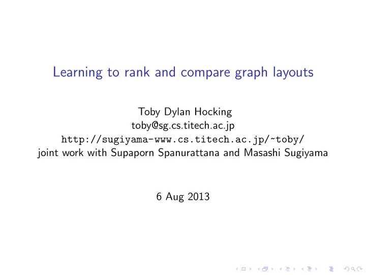
Learning to rank and compare graph layouts Toby Dylan Hocking toby@sg.cs.titech.ac.jp http://sugiyama-www.cs.titech.ac.jp/~toby/ joint work with Supaporn Spanurattana and Masashi Sugiyama 6 Aug 2013

Introduction: what makes a graph layout good or bad? Learning to rank and compare graph layouts

Biology is full of networks (graphs) Source: Kyoto encyclopedia of genes and genomes (KEGG).

Biology is full of networks (graphs) Source: Wikipedia “Citric acid cycle.”

Goal: find a good layout for a particular graph Two categories of methods for graph layout ◮ Heuristic layout algorithms: ◮ Force-directed ◮ Hierarchical clustering (trees/dendrograms) ◮ Hive plots ◮ ... ◮ Manual layout using programs such as: ◮ Cytoscape/cytoscape.js ◮ Gephi ◮ Image processing: gimp/inkscape ◮ ...

Force-directed layout has many tuning parameters Source: Data-Driven Documents (D3) JavaScript visualization library (Bostock 2011). parameter min default max size ? 1 x 1 ? link distance 0 20 ∞ link strength 0 1 1 friction 0 0.9 1 charge −∞ -30 ∞ theta 0 0.8 ∞ gravity 0 0.1 ∞ Question: how to tune these parameters for a specific graph?

Manual layout using a GUI is time-consuming ◮ Try default parameters of several different algorithms. ◮ Play with tuning parameters, select a combination that looks good. ◮ Finally, refine the algorithm’s layout by dragging nodes to positions that look better. Goal: learn from a database of manually labeled graphs.

Manual layout using a GUI is time-consuming ◮ Try default parameters of several different algorithms. ◮ Play with tuning parameters, select a combination that looks good. ◮ Finally, refine the algorithm’s layout by dragging nodes to positions that look better. Goal: learn from a database of manually labeled graphs.

Pairwise comparison in the graph layout literature Source: Holten and van Wijk, “Force-Directed Edge Bundling for Graph Visualization,” EuroVis 2009.

Pairwise comparison in the graph layout literature Source: Muelder and Ma, “Rapid Graph Layout Using Space Filling Curves,” InfoVis 2008.

Pairwise comparison in the graph layout literature Source: Gorochowski et al. , “Using Aging to Visually Uncover Evolutionary Processes on Networks,” IEEE Trans. Viz 2012.

Introduction: what makes a graph layout good or bad? Learning to rank and compare graph layouts

Learning a comparison function We are given n training pairs ( G i , x i , x ′ i , y i ) where we have ◮ a graph G i , i ∈ R p of that graph (feature vectors), ◮ two layouts x i , x ′  − 1 if x i is better   ◮ a comparison y i = 0 if x i is as good as x ′ i  1 if x ′ i is better .  Goal: find a comparison function g : R p × R p → {− 1 , 0 , 1 } ◮ Symmetry: g ( x , x ′ ) = − g ( x ′ , x ). ◮ Good prediction with respect to the zero-one loss E : � � y i , g ( x i , x ′ � minimize E i ) g i ∈ test

Learning to rank and compare We will learn a ◮ Ranking function f : R p → R . Bigger means a better layout. ◮ Threshold t ∈ R + . A small difference | f ( x ′ ) − f ( x ) | ≤ t is not significant.  if f ( x ′ ) − f ( x ) < − t − 1   ◮ Comparison function g t ( x , x ′ ) = 0 if | f ( x ′ ) − f ( x ) | ≤ t  1 if f ( x ′ ) − f ( x ) > t .  The problem becomes n � � y i , g t ( x i , x ′ � minimize E i ) f , t i =1

Some labeled layouts of a 2-node graph good 1 good 2 good 3 200 150 100 50 bad 11 bad 12 bad 13 y 200 150 100 50 -300 -200 -100 0 -300 -200 -100 0 -300 -200 -100 0 x

Map 20 layouts x i ∈ R 2 to a feature space 1.6 1.2 label angle good 0.8 bad 0.4 0 100 200 300 distance

Generate 10 pairwise constraints x ′ i − x i ∈ R 2 1.6 1.2 label angle good 0.8 bad 0.4 0 100 200 300 distance

10 labeled difference vectors x ′ i − x i ∈ R 2 1 comparison y i angle -1 0 0 1 -1 -200 0 200 distance

All 190 labeled difference vectors x ′ i − x i ∈ R 2 1 comparison y i angle -1 0 0 1 -1 -200 0 200 distance

Max margin comparison function line margin decision 1 comparison y i angle -1 0 0 1 -1 constraint active f ( x ′ ) − f ( x ) = − 1 f ( x ′ ) − f ( x ) = 1 inactive -200 0 200 distance

g when switching train direction x i , x ′ Invariance of ˆ i line margin 1 decision comparison angle y i 0 -1 0 constraint -1 active inactive f ( x ′ ) − f ( x ) = − 1 f ( x ′ ) − f ( x ) = 1 -200 0 200 distance

Defining the margin Recall: for all pairs i ∈ { 1 , . . . , n } we have i ∈ R p and ◮ features x i , x ′ ◮ comparisons y i ∈ {− 1 , 0 , 1 } . We define ◮ Ranking function f ( x ) = w ⊺ x ∈ R . ◮ Threshold t = 1. ◮ Comparison function g 1 ( x , x ′ ) ∈ {− 1 , 0 , 1 } . y i = − 1 y i = 0 y i = 1 1 margin µ 0 -1 0 1 -1 0 1 -1 0 1 predicted rank difference f ( x ′ i ) − f ( x i )

Max margin comparison is a linear program (LP) For y ∈ {− 1 , 0 , 1 } , let I y = { i | y i = y } be the corresponding training indices. maximize µ ∈ R , w ∈ R p µ subject to µ ≤ 1 − | w ⊺ ( x ′ i − x i ) | , ∀ i ∈ I 0 µ ≤ − 1 + w ⊺ ( x ′ i − x i ) y i , ∀ i ∈ I 1 ∪ I − 1 . Note: if the optimal µ > 0 then the data are separable.

Related work: reject, rank, and rate ❳❳❳❳❳❳❳❳❳❳❳ Inputs single items x pairs of items x , x ′ Outputs y ∈ {− 1 , 1 } SVM SVMrank y ∈ {− 1 , 0 , 1 } Reject option this work ◮ PL Bartlett and MH Wegkamp. Classification with a reject option using a hinge loss. JMLR, 9:1823–1840, 2008. (statistical properties of the hinge loss) ◮ T Joachims. Optimizing search engines using clickthrough data. KDD 2002. (SVMrank) ◮ K Zhou et al. Learning to rank with ties. SIGIR 2008. (boosting, ties are more effective with more output values) ◮ R Herbrich et al. TrueSkill: a Bayesian skill rating system. NIPS 2006. (generalization of Elo for chess)

SVMrank is a quadratic program (QP) minimize w ⊺ w w ∈ R p subject to w ⊺ ( x ′ i − x i ) y i ≥ 1 , ∀ i ∈ I 1 ∪ I − 1 . line 4 margin f ( x ′ ) − f ( x ) = 0 decision 2 comparison y i angle -1 0 0 1 -2 constraint active f ( x ′ ) − f ( x ) = − 1 f ( x ′ ) − f ( x ) = 1 inactive -2 -1 0 1 2 distance

Conclusions and future work Learned a function f ( x ) for ranking a graph layout x . ◮ Features for good performance on real graphs? ◮ Tune layout algorithm parameters to maximize f . ◮ SVMrank is sufficient under what assumption?

Thank you! Supplementary slides appear after this one.

Layout evaluation metrics (features x i , x ′ i ) ◮ Number of crossing edges (smaller is better) ◮ Aspect ratio (closer to 1:1 is better?) ◮ Symmetry (more is better when the graph has symmetries) ◮ Edge length (small and less variable is better?) ◮ Angle between edge pairs (big is better?) ◮ Area of smallest bounding box (smaller is better to let small features be more legible) Source: http://en.wikipedia.org/wiki/Graph_drawing# Quality_measures