1 SVD applications: rank, column, row, and null spaces Rank : the - PDF document
Statistical Modeling and Analysis of Neural Data (NEU 560) Princeton University, Spring 2018 Jonathan Pillow Lecture 3A notes: SVD and Linear Systems 1 SVD applications: rank, column, row, and null spaces Rank : the rank of a matrix is equal to:
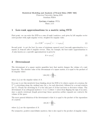
Statistical Modeling and Analysis of Neural Data (NEU 560) Princeton University, Spring 2018 Jonathan Pillow Lecture 3A notes: SVD and Linear Systems 1 SVD applications: rank, column, row, and null spaces Rank : the rank of a matrix is equal to: • number of linearly independent columns • number of linearly independent rows (Remarkably, these are always the same!). For an m × n matrix, the rank must be less than or equal to min( m, n ). The rank can be thought of as the dimensionality of the vector space spanned by its rows or its columns. Lastly, the rank of A is equal to the number of non-zero singular values! Consider the SVD of a matrix A that has rank k : A = USV ⊤ Column space: Since A is rank k , the first k left singular vectors, { � u k } (the columns of u 1 , . . . � U ), provide an orthonormal basis for the column space of A . Row space: Similarly, the first k right singular vectors, { � v 1 , . . .� v k } (the columns of V , or the rows of V ⊤ ), provide an orthonormal basis for the row space of A . Null space: The last right singular vectors, { � v k +1 , . . .� v n } (the last columns of V , or the last rows of V ⊤ ), provide an orthonormal basis for the null space of A . Let’s prove this last one, just to see what such a proof looks like. First, consider a vector � x that can be expressed as a linear combination of the last n − k columns of V : n � x = � w i � v i , i = k +1 for some real-valued weights { w i } . To show that � x lives in the null space of A , we need to show that A� x = 0. Let’s go ahead and do this now. (It isn’t that hard, and this gives the flavor of what a lot of proofs in linear algebra look like) 1
� n � � x = A (by definition of � x ) (1) A� w i � v i i = k +1 n � = w i ( A� v i ) . (by definition of linearity) (2) i = k +1 Now let’s look at any one of the terms in this sum: v i = ( USV ⊤ ) � v i = US ( V ⊤ � A� v i ) = US � e i , (3) where � e i is the “identity” basis vector consisting of all 0’s except for a single 1 in the i ’th row. v i is orthogonal to every row of V ⊤ except the i ’th row, which gives This follows from the fact that � � v i · � v i = 1 because � v i is a unit vector. Now, because i in the sum only ranged over k + 1 to n , then when we multiply � e i by S (which has non-zeros along the diagonal only up to the k ’th row / column), we get zero: e i = 0 for i > k. S� Thus US� e i = 0 which means that the entire sum n � US� e i = 0 . i = k +1 So this shows that A� x = 0 for any vector � x that lives in the subspace spanned by the last n − k columns of V , meaning it lies in the null space. This is of course equivalent to showing that the last n − k columns of V provide an (orthonormal) basis for the null space! 2 Positive semidefinite matrix Positive semi-definite (PSD) matrix is a matrix that has all eignevalues ≥ 0, or equivalently, x ⊤ A� a matrix A for which � x ≥ 0 for any vector � x . To generate an n × n positive semi-definite matrix, we can take any matrix X that has n columns and let A = X ⊤ X . 3 Relationship between SVD and eigenvector decomposition Definition : An eigenvector of a square matrix A is defined as a vector satisfying the equation x = λ� A� x, 2
and λ is the corresponding eigenvalue . In other words, an eigenvector of A is any vector that, when multiplied by A , comes back as itself scaled by λ . Spectral theorem : If a matrix A is symmetric and positive semi-definite, then the SVD also an eigendecomposition, that is, a decomposition in terms of an orthonormal basis of eigenvectors: A = USU ⊤ , where the columns of U are eigenvectors and the diagonal entries { s i } of S are the eigenvalues. Note that for such matrices, U = V , meaning the left and right singular vectors are identical. Exercise: prove to yourself that: A� u i = s i � u i In class we showed that if A = USV ⊤ , then A ⊤ A SVD of matrix times its transpose . (which it turns out, is symmetric and PSD) has the singular value decomposition (which is also an eigendecomposition): A ⊤ A = V S 2 V ⊤ . Test yourself by deriving the SVD of AA ⊤ . 4 Linearity and Linear Systems Linear system is a kind of mapping f ( � x ) − → � y that has the following two properties: 1. homogeneity (“scalar multiplication”): f ( ax ) = af ( x ) 2. additivity: f ( � x 1 + � x 2 ) = f ( � x 1 ) + f ( � x 2 ) Of course we can combine these two properties into a single requirement and say: f is a linear function if and only if it obeys the principal of superposition: f ( a� x 1 + b� x 2 ) = af ( � x 1 ) + bf ( � x 2 ) . General rule : we can write any linear function in terms of a matrix operation: f ( � x ) = A� x for some matrix A . Question : is the function f ( x ) = ax + b a linear function? Why or why not? 3
Recommend
More recommend
Explore More Topics
Stay informed with curated content and fresh updates.


