LEARNING SPARSE NEURAL NETWORKS THROUGH L0 REGULARIZATION Christos - PowerPoint PPT Presentation
LEARNING SPARSE NEURAL NETWORKS THROUGH L0 REGULARIZATION Christos Louizos, Max Welling, Diederik P. Kingma STA 4273 Paper Presentation Daniel Flam-Shepherd, Armaan Farhadi & Zhaoyu Guo March 2nd, 2018 1 / 14 Neural Networks: the good and
LEARNING SPARSE NEURAL NETWORKS THROUGH L0 REGULARIZATION Christos Louizos, Max Welling, Diederik P. Kingma STA 4273 Paper Presentation Daniel Flam-Shepherd, Armaan Farhadi & Zhaoyu Guo March 2nd, 2018 1 / 14
Neural Networks: the good and the bad Neural Networks : ... 1 are flexible function approximators that scale really well 2 are overparameterized and prone to overfitting and memorization So what can we do about this? Model compression and sparsification! Consider the Empirical Risk minimization problem N R ( θ ) = 1 � min L ( f ( x i ; θ ) , y i ) + λ || θ || p N θ i =1 where 1 { ( x i , y i ) } N i =1 is the iid dataset of input-output pairs 2 f ( x ; θ ) is the NN using parameters θ 3 || θ || p is the L p norm 4 L ( · ) is the loss function 2 / 14
Lp Norms Figure: L p norm penalties for parameter θ from lousizos et al The L 0 ”norm” is just the number of nonzero parameters. | θ | � || θ || 0 = I [ θ j � = 0] j =1 This does not impose shrinkage on large θ j rather it directly penalizes | θ | . 3 / 14
Reparameterizing If we use the L p norm R ( θ ) is non-differentiable at 0. How can we relax this optimization and ensure 0 ∈ θ ? First, Reparameterize by putting binary gates z j on each θ j . | θ | θ j = ˜ ˜ � θ j z j , z j ∈ { 0 , 1 } , θ j � = 0 , & || θ || 0 = z j j =1 let z j ∼ Ber( π j ) with pmf q ( z j | π j ) and we can formulate the problem as: | θ | � N � 1 θ , π R (˜ � L ( f ( x i ; ˜ � min θ , π ) = E q ( z | π ) θ ⊙ z ) , y i ) + λ π j N ˜ i =1 j =1 we cannot optimize the first term. 4 / 14
Smooth the objective so we can optimize it! Let gates z be given by a hard-sigmoid rectification of s , as follows z = g ( s ) = min( 1 , max( 0 , s )) , s ∼ q φ ( s ) The probability of a gate being active is q φ ( z � = 0) = 1 − Q φ ( s ≤ 0 ) Then using the reparametrization trick on s = f ( φ , ǫ ) so z = g ( f ( φ , ǫ )) | θ | � N � 1 � L ( f ( x i ; ˜ � min θ ⊙ g ( f ( φ , ǫ ))) , y i ) + λ 1 − Q φ ( s j ≤ 0) θ , φ E p ( ǫ ) N ˜ i =1 j =1 Okay but which distribution q φ ( s ) should we use? 5 / 14
Hard Concrete Distribution An appropriate smoothing distribution q ( s ) is the binary concrete rv s : u ∼ U (0 , 1) , s = Sigmoid ((log u − log(1 − u ) + log α ) /β )) s = s ( ζ − γ ) + γ and z = min(1 , max(0 , s )) 1 s is a concrete binary distributed 2 α is the location parameter, and 3 β is the temperature parameter 4 z is the hard concrete distribution. 5 we stretch s → ¯ s into the range ( γ, ζ ) where ζ < 0 and γ > 1. 6 / 14
Figure: Figure 2 from lousizos et al 7 / 14
Hard Concrete Distribution From earlier, we had 1 − Q φ ( s ≤ 0 ) in L 0 complexity loss of the objective function. Now, if the random variable is hard concrete, then we can say: 1 − Q φ ( s ≤ 0 ) = Sigmoid(log α − β log − γ ζ ) During test time, the authors use the following for the gate: z = min( 1 , max( 0 , Sigmoid(log α )( ζ − γ ) + γ )) and θ ∗ = ˜ θ ∗ ⊙ ˆ ˆ z 8 / 14
Experiments - MNIST Classification and Sparsification 9 / 14
Experiments - MNIST Classification Figure: Expected FLOPs. Left is the MLP. Right is the LeNet-5 10 / 14
Experiments - CIFAR Classification 11 / 14
Experiments - CIFAR Classification Figure: Expected FLOPs of WRN at CIFAR 10 (left) & 100 (right) 12 / 14
Discussion & Future Work Discussion 1 L 0 penalty can save memory and computation 2 L 0 regularization lead to competitive predictive accuracy and stability Future Work 1 Adopt a full Bayesian treatment over the parameter θ 13 / 14
Thank You . . . 14 / 14
Recommend
More recommend
Explore More Topics
Stay informed with curated content and fresh updates.
