Latent Variable Models Volodymyr Kuleshov Cornell Tech Lecture 5 - PowerPoint PPT Presentation
Latent Variable Models Volodymyr Kuleshov Cornell Tech Lecture 5 Volodymyr Kuleshov (Cornell Tech) Deep Generative Models Lecture 5 1 / 35 Announcements Glitches with Google Hangout link should be resolved. Will be checking email at the
Latent Variable Models Volodymyr Kuleshov Cornell Tech Lecture 5 Volodymyr Kuleshov (Cornell Tech) Deep Generative Models Lecture 5 1 / 35
Announcements Glitches with Google Hangout link should be resolved. Will be checking email at the beginning of each office hours session to make sure there are no more glitches. Homework template is available. Extra lecture notes have been posted. Good luck with ICML deadline! Volodymyr Kuleshov (Cornell Tech) Deep Generative Models Lecture 5 2 / 35
Recap of last lecture 1 Autoregressive models: Chain rule based factorization is fully general Compact representation via conditional independence and/or neural parameterizations 2 Autoregressive models Pros: Easy to evaluate likelihoods Easy to train 3 Autoregressive models Cons: Requires an ordering Generation is sequential Cannot learn features in an unsupervised way Volodymyr Kuleshov (Cornell Tech) Deep Generative Models Lecture 5 3 / 35
Plan for today 1 Latent variable models Definition Motivation 2 Warm-up: Shallow mixture models 3 Deep latent-variable models Representation: Variational autoencoder Learning: Variational inference Volodymyr Kuleshov (Cornell Tech) Deep Generative Models Lecture 5 4 / 35
Latent Variable Models: Motivation 1 Lots of variability in images x due to gender, eye color, hair color, pose, etc. However, unless images are annotated, these factors of variation are not explicitly available (latent). 2 Idea : explicitly model these factors using latent variables z Volodymyr Kuleshov (Cornell Tech) Deep Generative Models Lecture 5 5 / 35
Latent Variable Models: Definition A latent variable model defines a probability distribution p ( x , z ) = p ( x | z ) p ( z ) containing two sets of variables: 1 Observed variables x that represent the high-dimensional object we are trying to model. 2 Latent variables z that are not in the training set, but that are associated with the x via p ( z | x ) and can encode the structure of the data. Volodymyr Kuleshov (Cornell Tech) Deep Generative Models Lecture 5 6 / 35
Latent Variable Models: Example 1 Only shaded variables x are observed in the data (pixel values) 2 Latent variables z correspond to high level features If z chosen properly, p ( x | z ) could be much simpler than p ( x ) If we had trained this model, then we could identify features via p ( z | x ), e.g., p ( EyeColor = Blue | x ) 3 Challenge: Very difficult to specify these conditionals by hand Volodymyr Kuleshov (Cornell Tech) Deep Generative Models Lecture 5 7 / 35
Deep Latent Variable Models: Example 1 z ∼ N (0 , I ) 2 p ( x | z ) = N ( µ θ ( z ) , Σ θ ( z )) where µ θ ,Σ θ are neural networks 3 Hope that after training, z will correspond to meaningful latent factors of variation ( features ). Unsupervised representation learning. 4 As before, features can be computed via p ( z | x ). In practice, we will need to use approximate inference . Volodymyr Kuleshov (Cornell Tech) Deep Generative Models Lecture 5 8 / 35
Mixture of Gaussians: a Shallow Latent Variable Model Mixture of Gaussians. Bayes net: z → x . 1 z ∼ Categorical (1 , · · · , K ) 2 p ( x | z = k ) = N ( µ k , Σ k ) Generative process 1 Pick a mixture component k by sampling z 2 Generate a data point by sampling from that Gaussian Volodymyr Kuleshov (Cornell Tech) Deep Generative Models Lecture 5 9 / 35
Mixture of Gaussians: a Shallow Latent Variable Model Mixture of Gaussians: 1 z ∼ Categorical (1 , · · · , K ) 2 p ( x | z = k ) = N ( µ k , Σ k ) 3 Clustering: The posterior p ( z | x ) identifies the mixture component 4 Unsupervised learning: We are hoping to learn from unlabeled data (ill-posed problem) Volodymyr Kuleshov (Cornell Tech) Deep Generative Models Lecture 5 10 / 35
Representational Power of Mixture models Combine simple models into a more complex and expressive one K � � � p ( x ) = p ( x , z ) = p ( z ) p ( x | z ) = p ( z = k ) N ( x ; µ k , Σ k ) � �� � z z k =1 component The likelihood is non-convex: this increases representational power, but makes inference more challenging. Volodymyr Kuleshov (Cornell Tech) Deep Generative Models Lecture 5 11 / 35
Example: Unsupervised learning over hand-written digits Unsupervised clustering of handwritten digits. Volodymyr Kuleshov (Cornell Tech) Deep Generative Models Lecture 5 12 / 35
Example: Unsupervised learning over DNA sequence data Volodymyr Kuleshov (Cornell Tech) Deep Generative Models Lecture 5 13 / 35
Example: Unsupervised learning over face images Volodymyr Kuleshov (Cornell Tech) Deep Generative Models Lecture 5 14 / 35
Plan for today 1 Latent variable models Definition Motivation 2 Warm-up: Shallow mixture models 3 Deep latent-variable models Representation: Variational autoencoder Learning: Variational inference Volodymyr Kuleshov (Cornell Tech) Deep Generative Models Lecture 5 15 / 35
Variational Autoencoder A mixture of an infinite number of Gaussians: 1 z ∼ N (0 , I ) 2 p ( x | z ) = N ( µ θ ( z ) , Σ θ ( z )) where µ θ ,Σ θ are neural networks µ θ ( z ) = σ ( A z + c ) = ( σ ( a 1 z + c 1 ) , σ ( a 2 z + c 2 )) = ( µ 1 ( z ) , µ 2 ( z )) � � exp( σ ( b 1 z + d 1 )) 0 Σ θ ( z ) = diag (exp( σ ( B z + d ))) = 0 exp( σ ( b 2 z + d 2 )) θ = ( A , B , c , d ) 3 Even though p ( x | z ) is simple, the marginal p ( x ) is very complex/flexible Volodymyr Kuleshov (Cornell Tech) Deep Generative Models Lecture 5 16 / 35
Benefits of the Latent-Variable Approach Allow us to define complex models p ( x ) in terms of simple building blocks p ( x | z ) Natural for unsupervised learning tasks (clustering, unsupervised representation learning, etc.) No free lunch: much more difficult to learn compared to fully observed, autoregressive models Volodymyr Kuleshov (Cornell Tech) Deep Generative Models Lecture 5 17 / 35
Partially observed data Suppose that our joint distribution is p ( X , Z ; θ ) We have a dataset D , where for each datapoint the X variables are observed (e.g., pixel values) and the variables Z are never observed (e.g., cluster or class id.). D = { x (1) , · · · , x ( M ) } . Maximum likelihood learning: � � � � log p ( x ; θ ) = log p ( x ; θ ) = log p ( x , z ; θ ) x ∈D x ∈D x ∈D z Evaluating log � z p ( x , z ; θ ) can be hard! Volodymyr Kuleshov (Cornell Tech) Deep Generative Models Lecture 5 18 / 35
Example: Learning with Missing Values Suppose some pixel values are missing at train time (e.g., top half) Let X denote observed random variables, and Z the unobserved ones (also called hidden or latent) Suppose we have a model for the joint distribution (e.g., PixelCNN) p ( X , Z ; θ ) What is the probability p ( X = ¯ x ; θ ) of observing a training data point ¯ x ? � � p ( X = ¯ x , Z = z ; θ ) = p (¯ x , z ; θ ) z z Need to consider all possible ways to complete the image (fill green part) Volodymyr Kuleshov (Cornell Tech) Deep Generative Models Lecture 5 19 / 35
Example: Variational Autoencoder A mixture of an infinite number of Gaussians: z ∼ N (0 , I ). p ( x | z ) = N ( µ θ ( z ) , Σ θ ( z )) where µ θ ,Σ θ are neural networks Z are unobserved at train time (also called hidden or latent) Suppose we have a model for the joint distribution. What is the probability p ( X = ¯ x ; θ ) of observing a training data point ¯ x ? � � p ( X = ¯ x , Z = z ; θ ) d z = p (¯ x , z ; θ ) d z z z Volodymyr Kuleshov (Cornell Tech) Deep Generative Models Lecture 5 20 / 35
Partially observed data Suppose that our joint distribution is p ( X , Z ; θ ) We have a dataset D , where for each datapoint the X variables are observed (e.g., pixel values) and the variables Z are never observed (e.g., cluster or class id.). D = { x (1) , · · · , x ( M ) } . Maximum likelihood learning: � � � � log p ( x ; θ ) = log p ( x ; θ ) = log p ( x , z ; θ ) x ∈D x ∈D x ∈D z Evaluating log � z p ( x , z ; θ ) can be intractable. Suppose we have 30 binary latent features, z ∈ { 0 , 1 } 30 . Evaluating � z p ( x , z ; θ ) involves a sum with � 2 30 terms. For continuous variables, log z p ( x , z ; θ ) d z is often intractable. Gradients ∇ θ also hard to compute. Need approximations . One gradient evaluation per training data point x ∈ D , so approximation needs to be cheap. Volodymyr Kuleshov (Cornell Tech) Deep Generative Models Lecture 5 21 / 35
First attempt: Naive Monte Carlo Likelihood function p θ ( x ) for Partially Observed Data is hard to compute: 1 � � p θ ( x ) = p θ ( x , z ) = |Z| |Z| p θ ( x , z ) = |Z| E z ∼ Uniform ( Z ) [ p θ ( x , z )] All values of z z ∈Z We can think of it as an (intractable) expectation. Monte Carlo to the rescue: Sample z (1) , · · · , z ( k ) uniformly at random 1 Approximate expectation with sample average 2 k p θ ( x , z ) ≈ |Z| 1 � � p θ ( x , z ( j ) ) k z j =1 Works in theory but not in practice. For most z , p θ ( x , z ) is very low (most completions don’t make sense). Some are very large but will never ”hit” likely completions by uniform random sampling. Need a clever way to select z ( j ) to reduce variance of the estimator. Volodymyr Kuleshov (Cornell Tech) Deep Generative Models Lecture 5 22 / 35
Recommend
More recommend
Explore More Topics
Stay informed with curated content and fresh updates.
