AdaGeo: Adaptive Geometric Learning for Optimization and Sampling - PowerPoint PPT Presentation
AdaGeo: Adaptive Geometric Learning for Opti- mization and Sampling AdaGeo: Adaptive Geometric Learning for Optimization and Sampling Gabriele Abbati 1 , Alessandra Tosi 2 , Seth Flaxman 3 , Michael A Osborne 1 1 University of Oxford, 2
AdaGeo: Adaptive Geometric Learning for Opti- mization and Sampling AdaGeo: Adaptive Geometric Learning for Optimization and Sampling Gabriele Abbati 1 , Alessandra Tosi 2 , Seth Flaxman 3 , Michael A Osborne 1 1 University of Oxford, 2 Mind Foundry Ltd, 3 Imperial College London Afternoon Meeting on Bayesian Computation 2018 University of Reading
High-dimensional Problems AdaGeo: Adaptive • Gradient-based optimization • MCMC Sampling Geometric Learning for Opti- mization and Sampling Issues arising from high dimensionality: non-convexity strong correlations multimodality
Related Work AdaGeo: Adaptive Geometric Learning for Opti- Gradient-based optimization MCMC Sampling mization and Sampling AdaGrad Hamiltonian Monte Carlo AdaDelta Particle Monte Carlo Adam Stochastic gradient Langevin dynamics RMSProp All of these methods focus on computing clever updates for optimization algorithms or for Markov chains. Novelty : to the best of our knowledge, no dimensionality reduction approaches were applied in this direction before.
The Manifold Idea AdaGeo: Adaptive After t steps of optimization or sampling, we assume the obtained points in the Geometric Learning parameter space to be lying on a manifold . for Opti- mization and Sampling We then feed them to a dimensionality reduction method to find a lower-dimensional representation . 3D example : if the sampler/ optimizer algorithm keeps on returning proposals on a sphere surface, that information might be used to our advantage Can we perform better if the algorithm acts with knowledge of the manifold?
Latent Variable Models AdaGeo: Adaptive Geometric Learning Latent Variable Models describe a set Θ through a lower-dimensional latent set Ω for Opti- mization and Sampling Latent Variable Models map f Θ = { θ 1 , . . . , θ N ∈ R D } Ω = { ω 1 , . . . , ω N ∈ R Q } with Q < D where: - θ : observed variables/parameters - ω : latent variables - f : mapping - D , Q : dimensionalities of Θ and Ω respectively
Latent Variable Models AdaGeo: Adaptive Geometric Learning Latent Variable Models describe a set Θ through a lower-dimensional latent set Ω for Opti- mization and Sampling Latent Variable Models map f Θ = { θ 1 , . . . , θ N ∈ R D } Ω = { ω 1 , . . . , ω N ∈ R Q } with Q < D mapping: θ = f ( ω ) + η with η ∼ N ( 0 , β − 1 I ) Dimensionality reduction Manifold identification The lower-dimensional manifold on which the samples lie is characterized through the latent set
Gaussian Process Latent Variable Model AdaGeo: Adaptive Geometric Learning for Opti- mization The choice of the dimensionality reduction method fell on the Gaussian Process and Latent Variable Model [1] . Sampling GPLVM: Gaussian Process prior over mapping f in θ = f ( ω ) + η Motivation: Analytically sound mathematical tool Full distribution over the mapping f Full distribution over the derivatives of the mapping f [1] Lawrence, N., Probabilistic non-linear principal component analysis with Gaussian process latent variable models. Journal of machine learning research (2005)
Gaussian Process AdaGeo: Gaussian Process [2] : a collection of random variables, any finite number of which Adaptive Geometric have a joint Gaussian distribution. Learning for Opti- mization and If a real-valued stochastic process f is a GP , it will be denoted as Sampling f ( · ) ∼ GP ( m ( · ) , k ( · , · )) A Gaussian Process is fully specified by Training data a mean function m ( · ) Regression GP Real function a covariance function k ( · , · ) where m ( ω ) = E f ( ω ) [ ] , k ( ω , ω ′ ) = E f ( ω ) − m ( ω ) f ( ω ′ ) − m ( ω ′ ) [( )( )] [2] Rasmussen, C. E., Williams, C. K. I., Gaussian Processes for Machine Learning, the MIT Press (2006)
Gaussian Process Latent Variable Model AdaGeo: Adaptive Geometric GPLVM: Gaussian Process prior over mapping f in Learning for Opti- mization and θ = f ( ω ) + η Sampling The likelihood of the data Θ given the latent Ω is given by 1 marginalizing the mapping 2 optimizing the latent variables Resulting likelihood: D p ( Θ | Ω , β ) = ∏ θ : , j | 0 , K + β − 1 I ( ) N j =1 D ∏ θ : , j | 0 , ˜ K ( ) = N j =1 With the resulting noise model being: θ i , j = ˜ K ( ω i , Ω ) ˜ K − 1 Θ : , j + η j
Gaussian Process Latent Variable Model AdaGeo: Adaptive Geometric GPLVM: Gaussian Process prior over mapping f in Learning for Opti- mization and θ = f ( ω ) + η Sampling For differentiable kernels k ( · , · ) , the Jacobian J of the mapping f can be computed analytically: J ij = ∂ f i ∂ω j But as previously said, GPLVM can yield the full (Gaussian) distribution over the Jacobian. If the rows of J are assumed to be independent: D ∏ p ( J | Ω , β ) = J i , : | µ J i , : , Σ J ( ) N , i =1
Recap AdaGeo: Adaptive Geometric 1 After t iterations the optimization or sampling algorithm has yielded a set of Learning for Opti- observed points Θ = { θ 1 , . . . , θ N ∈ R D } in the parameter space mization and Sampling 2 A GPLVM is trained on Θ in order to build a latent space Ω that describes the lower-dimensional manifold on which the optimization/sampling is allegedly taking place. We can: - move from the latent space Ω to the observed space Θ : θ = f ( ω ) + η Θ ← Ω but not viceversa ( f is not invertible) - bring the gradients of a generic function g : Θ → R from the observed space Θ to the latent space Ω : ∇ ω g f ( ω ) = µ J ∇ θ g ( θ ) ( ) Ω ← Θ In this case a punctual estimate of J is given by the mean of its distribution.
Recap AdaGeo: Adaptive Geometric 1 After t iterations the optimization or sampling algorithm has yielded a set of Learning for Opti- observed points Θ = { θ 1 , . . . , θ N ∈ R D } in the parameter space mization and Sampling 2 A GPLVM is trained on Θ in order to build a latent space Ω that describes the lower-dimensional manifold on which the optimization/sampling is allegedly taking place. We can: - move from the latent space Ω to the observed space Θ : θ = f ( ω ) + η Θ ← Ω but not viceversa ( f is not invertible) - bring the gradients of a generic function g : Θ → R from the observed space Θ to the latent space Ω : ∇ ω g f ( ω ) = µ J ∇ θ g ( θ ) ( ) Ω ← Θ In this case a punctual estimate of J is given by the mean of its distribution.
Recap AdaGeo: Adaptive Geometric 1 After t iterations the optimization or sampling algorithm has yielded a set of Learning for Opti- observed points Θ = { θ 1 , . . . , θ N ∈ R D } in the parameter space mization and Sampling 2 A GPLVM is trained on Θ in order to build a latent space Ω that describes the lower-dimensional manifold on which the optimization/sampling is allegedly taking place. We can: - move from the latent space Ω to the observed space Θ : θ = f ( ω ) + η Θ ← Ω but not viceversa ( f is not invertible) - bring the gradients of a generic function g : Θ → R from the observed space Θ to the latent space Ω : ∇ ω g f ( ω ) = µ J ∇ θ g ( θ ) ( ) Ω ← Θ In this case a punctual estimate of J is given by the mean of its distribution.
Recap AdaGeo: Adaptive Geometric 1 After t iterations the optimization or sampling algorithm has yielded a set of Learning for Opti- observed points Θ = { θ 1 , . . . , θ N ∈ R D } in the parameter space mization and Sampling 2 A GPLVM is trained on Θ in order to build a latent space Ω that describes the lower-dimensional manifold on which the optimization/sampling is allegedly taking place. We can: - move from the latent space Ω to the observed space Θ : θ = f ( ω ) + η Θ ← Ω but not viceversa ( f is not invertible) - bring the gradients of a generic function g : Θ → R from the observed space Θ to the latent space Ω : ∇ ω g f ( ω ) = µ J ∇ θ g ( θ ) ( ) Ω ← Θ In this case a punctual estimate of J is given by the mean of its distribution.
AdaGeo Gradient-based Optimization AdaGeo: Adaptive Geometric Minimization problem: Learning θ ∗ = arg min for Opti- θ g ( θ ) mization and Sampling Iterative scheme solution (e.g. (stochastic) gradient descent): θ t +1 = θ t − ∆ θ t ( ∇ θ g ) We propose, after having learned a latent representation with GPLVM, to move the problem onto the latent space Ω Minimization problem: ω ∗ = arg min ω g ( f ( ω )) Iterative scheme solution (e.g. (stochastic) gradient descent): ω t +1 = ω t − ∆ ω t ( ∇ ω g )
AdaGeo Gradient-based Optimization AdaGeo: Adaptive Geometric Minimization problem: Learning θ ∗ = arg min for Opti- θ g ( θ ) mization and Sampling Iterative scheme solution (e.g. (stochastic) gradient descent): θ t +1 = θ t − ∆ θ t ( ∇ θ g ) We propose, after having learned a latent representation with GPLVM, to move the problem onto the latent space Ω Minimization problem: ω ∗ = arg min ω g ( f ( ω )) Iterative scheme solution (e.g. (stochastic) gradient descent): ω t +1 = ω t − ∆ ω t ( ∇ ω g )
Recommend
More recommend
Explore More Topics
Stay informed with curated content and fresh updates.
