1 Latent variable models In the next section we will discuss latent - PDF document

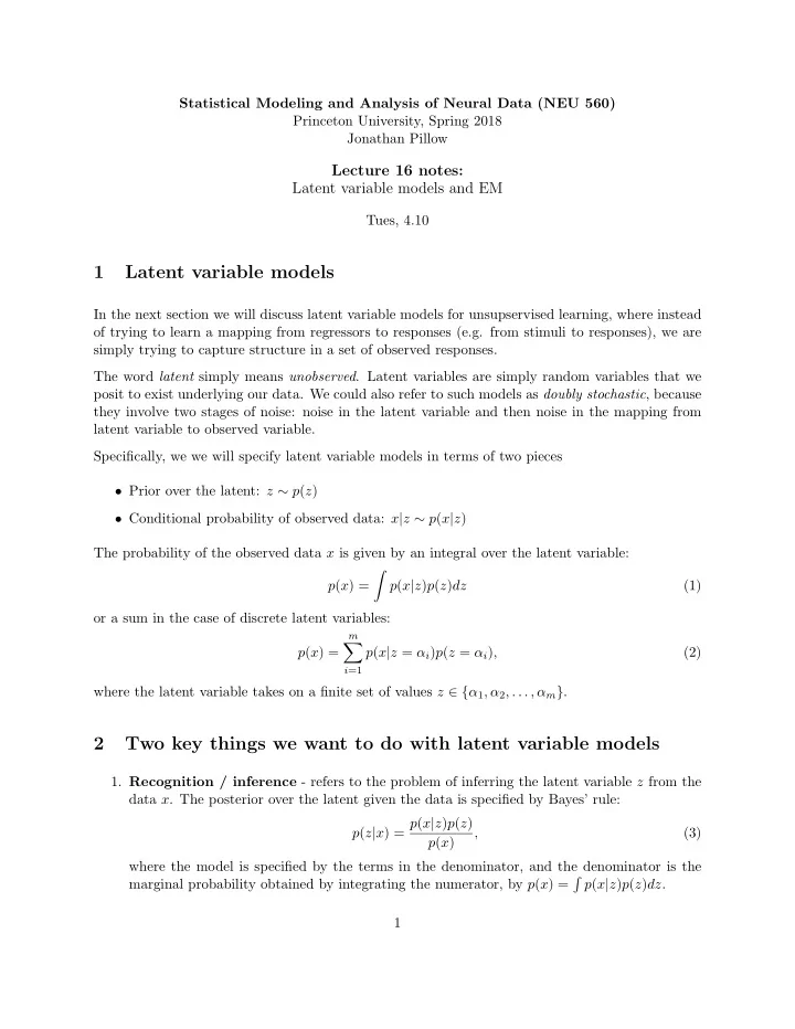
Statistical Modeling and Analysis of Neural Data (NEU 560) Princeton University, Spring 2018 Jonathan Pillow Lecture 16 notes: Latent variable models and EM Tues, 4.10 1 Latent variable models In the next section we will discuss latent variable models for unsupservised learning, where instead of trying to learn a mapping from regressors to responses (e.g. from stimuli to responses), we are simply trying to capture structure in a set of observed responses. The word latent simply means unobserved . Latent variables are simply random variables that we posit to exist underlying our data. We could also refer to such models as doubly stochastic , because they involve two stages of noise: noise in the latent variable and then noise in the mapping from latent variable to observed variable. Specifically, we we will specify latent variable models in terms of two pieces • Prior over the latent: z ∼ p ( z ) • Conditional probability of observed data: x | z ∼ p ( x | z ) The probability of the observed data x is given by an integral over the latent variable: � p ( x ) = p ( x | z ) p ( z ) dz (1) or a sum in the case of discrete latent variables: m � p ( x ) = p ( x | z = α i ) p ( z = α i ) , (2) i =1 where the latent variable takes on a finite set of values z ∈ { α 1 , α 2 , . . . , α m } . 2 Two key things we want to do with latent variable models 1. Recognition / inference - refers to the problem of inferring the latent variable z from the data x . The posterior over the latent given the data is specified by Bayes’ rule: p ( z | x ) = p ( x | z ) p ( z ) , (3) p ( x ) where the model is specified by the terms in the denominator, and the denominator is the � marginal probability obtained by integrating the numerator, by p ( x ) = p ( x | z ) p ( z ) dz . 1

2. Model fitting - refers to the problem of learning the model parameters, which we have so far suppressed. In fact we should write the model as specified by p ( x, z | θ ) = p ( x | z, θ ) p ( z | θ ) (4) where θ are the parameters governing both the prior over the latent and the conditional distribution of the data. Maximum likelihood fitting involves computing and maximizing the marginal probability: � ˆ θ = arg max p ( x | θ ) = arg max p ( x, z | θ ) dz. (5) θ θ 3 Example: binary mixture of Gaussians (MoG) (Also commonly known as a Gaussian mixture model (GMM) ). This model is specified by: z ∼ Ber( p ) (6) � N ( µ 0 , C 0 ) , if p = 0 x | z ∼ (7) N ( µ 1 , C 1 ) , if p = 1 So z is a binary random variable that takes value 1 with probability p and value 0 with probability (1 − p ). The datapoint x is then drawn from either Gaussian N 0 ( x ) = N ( µ 0 , C 0 ) if p = 0 or a different Gaussian N 1 ( x ) = N ( µ 1 , C 1 ) if p = 1. For this simple model the recognition distribution (conditional distribution of the latent): (1 − p ) N 0 ( x ) p ( z = 0 | x ) = (8) (1 − p ) N 0 ( x ) + p N 1 ( x ) p N 1 ( x ) p ( z = 1 | x ) = (9) (1 − p ) N 0 ( x ) + p N 1 ( x ) The likelihood (or marginal likelihood) is simply the normalizer in the expressions above: p ( x | θ ) = (1 − p ) N 0 ( x ) + p N 1 ( x ) , (10) where the model parameters are θ = { p, µ 0 , C 0 , µ 1 , C 1 } . For an entire dataset, likelihood would be the product of independent terms, since we assume each latent z i is drawn independently from the prior, giving: N � � � p ( X | θ ) = (1 − p ) N 0 ( x i ) + p N 1 ( x i ) (11) i =1 and hence N � � � log p ( X | θ ) = (1 − p ) N 0 ( x i ) + p N 1 ( x i ) log . (12) i =1 2

Clearly we could write a function to compute this sum and use an off-the-shelf algorithm to optimize it numerically if we wanted to. However, we will next discuss an alternative iterative approach to maximizing the likelihood. 4 The Expectation-Maximization (EM) algorithm 4.1 Jensen’s inequality Before we proceed to the algorithm, let’s first describe one of the tools used in its derivation. Jensen’s inequality : for any concave function f and p ∈ [0 , 1], f ((1 − p ) x 1 + px 2 ) ≥ (1 − p ) f ( x 1 ) + pf ( x 2 ) . (13) The left hand side is the function f evaluated at a point somewhere between x 1 and x 2 , while the right hand side is a point on the straight line (a chord) connecting f ( x 1 ) and f ( x 2 ). Since a concave function lies above any chord, this follows straightforwardly from the definition of concave functions. (For convex functions the inequality is reversed!) In our hands we will use the function f ( x ) = exp( x ), in which case we can think of Jensen’s inequality as equivalent to the statement that “The log of the average is greater than or equal to the average of the logs” . The inequality can be extended to any continuous probability distribution p ( x ) and implies that: � � f ( p ( x ) g ( x ) dx ≥ p ( x ) f ( g ( x )) dx (14) for any concave f ( x ), or in our case: � � log p ( x ) g ( x ) dx ≥ p ( x ) log g ( x ) . (15) 4.2 EM The expectation-maximization algorithm is an iterative method for finding the maximum likelihood estimate for a latent variable model. It consists of iterating between two steps (“Expectation step” and “Maximization step”, or “E-step” and “M-step” for short) until convergence. Both steps involve maximizing a lower bound on the likelihood. Before deriving this lower bound, recall that p ( x | z, θ ) p ( z | θ ) = p ( x, z | theta ) = p ( z | x, θ ) p ( x | θ ). This is a quantity known in the EM literature as the total data likelihood . The log-likelihood can be lower-bounded through a straightforward application of Jensen’s inequal- 3

ity: log p ( x | θ ) = log p ( x, z | θ ) dz (definition of log-likelihood) (16) = log q ( z | φ ) p ( x, z | θ ) (multiply and divde by q ) (17) q ( z | φ ) dz � � p ( x, z | θ ) � ≥ q ( z | φ ) log (apply Jensen) (18) dz q ( z | φ ) � F ( φ, θ ) (negative Free Energy) (19) Here q ( z | φ ) is an arbitrary distribution over the latent z , with parameters φ . The quantity we have obtained in equation (eq. 18) is known as the negative free energy F ( φ, θ ). We will now write the negative free energy in two different forms. First: � � p ( x, z | θ ) � F ( φ, θ ) = q ( z | φ ) log (20) dz q ( z | φ ) � p ( x | θ ) p ( z | x, θ ) � � q ( z | φ ) log = dz (21) q ( z | φ ) � p ( z | x, θ ) � � � = q ( z | φ ) log p ( x | θ ) + q ( z | φ ) log dz (22) q ( z | φ ) � � = log p ( x | θ ) − KL q ( z | φ ) || p ( z | x, θ ) (23) This last line makes clear that the NFE is indeed a lower bound on log p ( x | θ ) because the KL divergence is always non-negative. Moreover, it shows how to make the bound tight, namely by setting φ such that the q distribution is equal to the conditional distribution over the latent given the data and the current parameters θ , i.e., q ( z | φ ) = p ( z | x, θ ). A second way to write the NFE that will prove useful is: � � p ( x, z | θ ) � F ( φ, θ ) = q ( z | φ ) log (24) dz q ( z | φ ) � � = q ( z | φ ) log p ( x, z | θ ) dz − q ( z | φ ) log q ( z | φ ) dz. (25) Here we observe that the second term is independent of θ . We can therefore maximize the NFE for θ by simply maximizing the first term. We are now ready to define the two steps of the EM algorithm: • E-step : Update φ by setting q ( z | φ ) = p ( z | x, θ ) (eq. 23), with θ held fixed. � • M-step : Update θ by maximizing the expected total data likelihood, q ( z | φ ) log p ( x, z | θ ) dz (eq. 25), with φ held fixed. Note that the lower bound on the log-likelihood will be tight after each E-step. 4