Part III: Latent Tree Models Le Song ICML 2012 Tutorial on Spectral - PowerPoint PPT Presentation

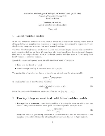
Spectral Algorithms for Latent Variable Models Part III: Latent Tree Models Le Song ICML 2012 Tutorial on Spectral Algorithms for Latent Variable Models, Edinburgh, UK Joint work with Mariya Ishteva, Ankur Parikh, Eric Xing, Byron Boots , Geoff Gordon, Alex Smola and Kenji Fukumizu

Latent Tree Graphical Models Graphical model: nodes represent variables, edges represent conditional independence relation Latent tree graphical models: latent and observed variables are arranged in a tree structure Latent Variable Observed Variable 𝑌 10 Latent Tree Hidden Markov Model 𝑌 7 𝑌 8 𝑌 9 𝑌 10 𝑌 11 𝑌 12 𝑌 7 𝑌 8 𝑌 9 𝑌 1 𝑌 2 𝑌 3 𝑌 4 𝑌 5 𝑌 6 𝑌 1 𝑌 2 𝑌 3 𝑌 4 𝑌 5 𝑌 6 Many real world applications, eg., time-series prediction, topic modeling 2

Scope of This Tutorial Estimating marginal probability of the observed variables Spectral HMMs (Hsu et al. COLT’09) Kernel spectral HMMs (Song et al. ICML’10) Spectral latent tree (Parikh et al. ICML’11, Song et al. NIPS’11) Spectral dimensional reduction for HMMs (Foster et al. Arxiv) More recent: Cohen et al. ACL’12, Balle et al. ICML’12 Estimating latent parameters PCA approach (Mossel & Roch AOAP’06) PCA and SVD approach, (Anandkumar et al. COLT’12, Arxiv) Estimating the structure of latent variable models Recursive grouping (Choi et al. JMLR’11) Spectral short quartet (Anandkumar et al. NIPS’11) 3

Challenge of Estimating Marginal of Observed Variables Exponential number of entries in 𝑄 𝑌 1 , 𝑌 2 , … , 𝑌 6 Discrete variable taking 𝑜 possible values, 𝑄 has 𝑃(𝑜 6 ) entries! Latent tree reduces the number of parameters 𝑄 𝑌 1 , 𝑌 2 , … , 𝑌 6 = 𝑄 𝑌 1 , 𝑌 2 , … , 𝑌 6 , 𝑦 7 , … , 𝑦 10 𝑃 3𝑜 2 𝑦 7 ,𝑦 8 ,𝑦 9 ,𝑦 10 𝑃 𝑜 params params 𝑄 𝑌 10 𝑄 𝑦 7 𝑦 10 𝑄 𝑌 1 𝑦 7 𝑄 𝑌 2 𝑦 7 𝑌 10 𝑦 7 ,𝑦 8 ,𝑦 9 ,𝑦 10 𝑄 𝑦 8 𝑦 10 𝑄 𝑌 3 𝑦 8 𝑄(𝑌 4 |𝑦 8 ) 𝑄 𝑦 9 𝑦 10 𝑄 𝑌 5 𝑦 9 𝑄(𝑌 6 |𝑦 9 ) 𝑌 9 𝑌 7 𝑌 8 Latent tree has 𝑃 9𝑜 2 params 𝑌 1 𝑌 2 𝑌 3 𝑌 4 𝑌 5 𝑌 6 Significant saving! 4

EM Algorithm for Parameter Estimation Do not observe latent variables, need to estimate the corresponding parameters, eg., 𝑄(𝑌 7 |𝑌 10 ) and 𝑄 𝑌 1 𝑌 7 𝑌 10 Goal of spectral algorithm: 𝑌 7 𝑌 8 𝑌 9 Estimate the marginal in 𝑌 1 𝑌 2 𝑌 3 𝑌 4 𝑌 5 𝑌 6 local-minimum-free fashion 1 1 1 1 1 1 𝑗 = 1 𝑦 1 𝑦 2 𝑦 3 𝑦 4 𝑦 6 𝑦 5 … … … 𝑛 𝑛 𝑛 𝑛 𝑛 𝑛 𝑗 = 𝑛 𝑦 2 𝑦 3 𝑦 1 𝑦 4 𝑦 5 𝑦 6 Expectation maximization: maximize likelihood of observations 𝑛 𝑗 , … , 𝑦 6 𝑗 ) max 𝑄(𝑦 1 𝑗=1 Drawback: local maxima, slow to converge, difficult to analyze 5

Key Features of Spectral Algorithms Represent joint probability table of observed variables with low rank factorization, without using the joint table in the computation! Eg. 𝑄 1,…,𝑒 ; 𝑒+1 ,…,2𝑒 = 𝑆𝑓𝑡ℎ𝑏𝑞𝑓(𝑄 𝑌 1 , … , 𝑌 2𝑒 , 1, … , 𝑒 ) 𝑜 𝑒 • Represent it by low rank factors to avoid exponential blowup • Use clever decomposition 𝑜 𝑒 𝑄 1,…,𝑒 ; 𝑒+1 ,…,2𝑒 technique to avoid directly using all entries from the table • Use singular value decomposition 6

Tensor View of Marginal Probability Marginal probability table 𝓤 = 𝑄 𝑌 1 , 𝑌 2 , … , 𝑌 6 Discrete variable taking 𝑜 possible values 1, … , 𝑜 6-way table, or 6 th order tensor Dimension labeled by the variable Value of the variable is the index to the corresponding dimension, need 6 indexes to access a single entry 𝑄(𝑌 1 = 1, 𝑌 2 = 4, … , 𝑌 6 = 3) is the entry 𝓤[1,4, … , 3] Running Examples: Latent Tree 𝑌 10 𝑌 7 𝑌 8 𝑌 9 𝑌 10 𝑌 11 𝑌 12 Hidden Markov 𝑌 7 𝑌 8 𝑌 9 Model 𝑌 1 𝑌 2 𝑌 3 𝑌 4 𝑌 5 𝑌 6 𝑌 1 𝑌 2 𝑌 3 𝑌 4 𝑌 5 𝑌 6 7

Reshaping Tensor into Matrices 𝑈 = 𝑆𝑓𝑡ℎ𝑏𝑞𝑓 𝓤, 𝒟 : multi-index 𝒟 mapped into row index, and the remaining indexes into column index Eg. 𝓤 = 𝑄 𝑌 1 , 𝑌 2 , 𝑌 3 , a 3 rd order tensor and 𝑜 = 3 𝑄 2 ;{1,3} = 𝑆𝑓𝑡ℎ𝑏𝑞𝑓 𝓤, {2} turns the dimension of 𝑌 2 into row 𝑌 3 𝑌 1 𝑌 1 Slice at dimension of 𝑌 3 𝑌 2 𝑌 2 𝓤 𝑌 3 = 1 𝑌 3 = 2 𝑌 3 = 3 𝑌 1 𝑈 = 𝑌 2 8

Reshaping 6 th Order Tensor 𝑈 = 𝑄 1,2,3 ;{4,5,6} = 𝑆𝑓𝑡ℎ𝑏𝑞𝑓(𝑄 𝑌 1 , … , 𝑌 6 , 1,2,3 ) 𝑌 6 1 1 1 1 1 1 1 1 1 2 2 2 2 2 2 2 2 2 3 3 3 3 3 3 3 3 3 𝑌 5 1 1 1 2 2 2 3 3 3 1 1 1 2 2 2 3 3 3 1 1 1 2 2 2 3 3 3 𝑌 4 1 2 3 1 2 3 1 2 3 1 2 3 1 2 3 1 2 3 1 2 3 1 2 3 1 2 3 𝑌 1 𝑌 3 𝑌 2 1 1 1 1 1 1 1 1 1 2 2 2 2 2 2 2 2 2 3 3 3 3 3 3 3 3 3 1 2 3 1 2 3 1 2 3 1 2 3 1 2 3 1 2 3 1 2 3 1 2 3 1 2 3 1 1 1 2 2 2 3 3 3 1 1 1 2 2 2 3 3 3 1 1 1 2 2 2 3 3 3 Each entry is the probability of a unique assignment to 𝑄(2,3,1,2,1,2) 𝑌 1 , … , 𝑌 6 9

Reshaping according to Latent Tree Structure For marginal 𝓠 = 𝑄 𝑌 1 , 𝑌 2 , … , 𝑌 6 of a latent tree model, reshape it according to the edges in the tree 𝑄 1 ;{2,3,4,5,6} = 𝑆𝑓𝑡ℎ𝑏𝑞𝑓(𝓠, 1 ) 𝑌 10 𝑌 9 𝑌 7 𝑌 8 𝑄 1,2 ;{3,4,5,6} = 𝑆𝑓𝑡ℎ𝑏𝑞𝑓(𝓠, 1,2 ) 𝑌 1 𝑌 2 𝑌 3 𝑌 4 𝑌 5 𝑌 6 𝑄 1 ;{2,3,4,5,6} 𝑄 1,2,3,4 ;{5,6} = 𝑆𝑓𝑡ℎ𝑏𝑞𝑓(𝓠, 1,2,3,4 ) 𝑌 10 𝑌 10 𝑌 7 𝑌 8 𝑌 9 𝑌 7 𝑌 8 𝑌 9 𝑌 1 𝑌 2 𝑌 3 𝑌 4 𝑌 5 𝑌 6 𝑌 1 𝑌 2 𝑌 3 𝑌 4 𝑌 5 𝑌 6 𝑄 1,2 ;{3,4,5,6} 𝑄 1,2,3,4 ;{5,6} 10

Low Rank Structure after Reshaping Size of 𝑄 1,2 ;{3,4,5,6} is 𝑜 2 × 𝑜 4 , but its rank is just 𝑜 𝑌 10 𝑄 𝑌 1 , 𝑌 2 , … , 𝑌 6 = 𝑌 9 𝑌 7 𝑌 8 𝑄 𝑌 1 , 𝑌 2 𝑦 7 𝑄 𝑦 7 , 𝑦 10 𝑌 1 𝑌 2 𝑌 3 𝑌 4 𝑌 5 𝑌 6 𝑦 7 ,𝑦 10 𝑄(𝑌 3 , 𝑌 4 , 𝑌 5 , 𝑌 6 |𝑦 10 ) 𝑄 1,2 ;{3,4,5,6} Use matrix multiplications to express summation over 𝑌 7 , 𝑌 10 ⊤ 𝑄 1,2 ;{3,4,5,6} = 𝑄 1,2 | 7 𝑄 7 ;{10} 𝑄 3,4,5,6 |{10} 𝑄 1,2 | 7 ≔ 𝑆𝑓𝑡ℎ𝑏𝑞𝑓(𝑄 𝑌 1 , 𝑌 2 𝑌 7 , 1,2 ) 𝑄 3,4,5,6 | 10 ≔ 𝑆𝑓𝑡ℎ𝑏𝑞𝑓(𝑄 𝑌 3 , 𝑌 4 , 𝑌 5 , 𝑌 6 𝑌 10 , 3,4,5,6 ) 𝑜 4 𝑜 4 𝑜 𝑜 𝑜 𝑜 𝑜 2 𝑜 2 = 𝑄 1,2 ;{3,4,5,6} 𝑄 7 ;{10} 11

Low Rank Structure of Latent Tree Model ⊤ 𝑄 3,4 ;{1,2,5,6} = 𝑄 3,4 | 8 𝑄 8 ;{10} 𝑄 1,2,5,6 |{10} 𝑜 4 𝑜 4 𝑜 𝑜 𝑜 𝑜 𝑜 2 = 𝑜 2 ⊤ 𝑄 1 ;{2,3,4,5,6} = 𝑄 1 | 7 𝑄 7 ;{7} 𝑄 2,3,4,5,6 |{7} 𝑜 5 = 𝑜 𝑜 5 𝑜 𝑜 𝑜 𝑜 𝑜 𝑌 10 𝑌 9 𝑌 7 𝑌 8 All these reshapings are low rank, and with rank 𝑜 𝑌 1 𝑌 2 𝑌 3 𝑌 4 𝑌 5 𝑌 6 12

Low Rank Structure of Hidden Markov Models 𝑌 7 𝑌 8 𝑌 9 𝑌 10 𝑌 11 𝑌 12 𝑌 1 𝑌 2 𝑌 3 𝑌 4 𝑌 5 𝑌 6 ⊤ 𝑄 1,2 ;{3,4,5,6} = 𝑄 1,2 | 8 𝑄 8 ;{9} 𝑄 3,4,5,6 |{9} 𝑜 4 𝑜 4 𝑜 𝑜 𝑜 𝑜 𝑜 2 = 𝑜 2 ⊤ 𝑄 1,2,3 ;{4,5,6} = 𝑄 1,2,3 | 9 𝑄 9 ;{10} 𝑄 4,5,6 |{10} 𝑜 3 𝑜 3 𝑜 𝑜 𝑜 𝑜 = 𝑜 3 𝑜 3 13

Key Features of Spectral Algorithms Represent joint probability table of observed variables with low rank factorization, without using the joint table in the computation! Eg. 𝑄 1,…,𝑒 ; 𝑒+1 ,…,2𝑒 = 𝑆𝑓𝑡ℎ𝑏𝑞𝑓(𝑄 𝑌 1 , … , 𝑌 2𝑒 , 1, … , 𝑒 ) 𝑜 𝑒 • Represent it by low rank factors to avoid exponential blowup • Use clever decomposition 𝑜 𝑒 𝑄 1,…,𝑒 ; 𝑒+1 ,…,2𝑒 technique to avoid directly using all entries from the table • Use singular value decomposition 14

Key Theorem Theorem 1: 𝑄: 𝑡𝑗𝑨𝑓 𝑛 × 𝑜, 𝑠𝑏𝑜𝑙 𝑙 𝐵: 𝑡𝑗𝑨𝑓 𝑜 × 𝑙, 𝑠𝑏𝑜𝑙 𝑙 𝐶: 𝑡𝑗𝑨𝑓 𝑙 × 𝑛, 𝑠𝑏𝑜𝑙 𝑙 𝐶𝑄𝐵 −1 𝐶𝑄 𝐽𝑔 𝐶𝑄𝐵 𝑗𝑜𝑤𝑓𝑠𝑢𝑗𝑐𝑚𝑓, 𝑢ℎ𝑓𝑜 𝑄 = 𝑄𝐵 𝑄 will be the reshaped joint probability table 𝐵 and 𝐶 will be marginalization operator Theorem 1 will be applied recursively Recover several existing spectral algorithms as special cases 15

Marginalization Operator A and B Compute the marginal probability of a subset of variables can be expressed as matrix product 𝑄 𝑌 1 , 𝑌 2 , 𝑌 3 , 𝑌 4 = 𝑄 𝑌 1 , 𝑌 2 , 𝑌 3 , 𝑌 4 , 𝑦 5 , 𝑦 6 𝑦 5 ,𝑦 6 𝑄 1,2,3 ; 4 = 𝑄 1,2,3 ;{4,5,6} 𝐵 , where 𝐵 = 1 𝑜 ⊗ 1 𝑜 ⊗ 𝐽 𝑜 𝑜 3 𝑜 𝑜 𝑜 1 1 𝑜 ⊗ ⊗ 𝑜 𝑜 𝑜 𝐽 𝑜 3 𝑜 3 𝑜 3 = 𝑜 3 = 𝐵 𝐵 1 𝑜 2 16

Zoom into Marginalization Operation 𝑌 6 1 1 1 1 1 1 1 1 1 2 2 2 2 2 2 2 2 2 3 3 3 3 3 3 3 3 3 𝑌 5 1 1 1 2 2 2 3 3 3 1 1 1 2 2 2 3 3 3 1 1 1 2 2 2 3 3 3 𝑌 4 1 2 3 1 2 3 1 2 3 1 2 3 1 2 3 1 2 3 1 2 3 1 2 3 1 2 3 = 𝑄 1,2,3 ;{4} 𝑄 1,2,3 ;{4,5,6} 1 3 ⊗ 1 3 ⊗ 𝐽 3 17

Apply Theorem 1 to Latent Tree Model Let 𝑌 10 𝑄 = 𝑄 1,2 ;{3,4,5,6} 𝑌 9 𝐵 = 1 𝑜 ⊗ 1 𝑜 ⊗ 1 𝑜 ⊗ 𝐽 𝑜 𝑌 7 𝑌 8 𝐶 = 𝐽 𝑜 ⊗ 1 𝑜 ⊤ 𝑌 1 𝑌 2 𝑌 3 𝑌 4 𝑌 5 𝑌 6 𝑄 1,2 ;{3,4,5,6} Then 𝑄 1,2 ; 3,4,5,6 𝐵 = 𝑄 1,2 ;{3} 𝐶𝑄 1,2 ; 3,4,5,6 = 𝑄 2 ;{3,4,5,6} 𝐶𝑄 1,2 ; 3,4,5,6 𝐵 = 𝑄 2 ;{3} 𝐶𝑄𝐵 −1 𝐶𝑄 Finally use 𝑄 = 𝑄𝐵 −1 𝑄 1,2 ;{3,4,5,6} = 𝑄 1,2 ;{3} 𝑄 2 ; 3 𝑄 2 ;{3,4,5,6} 18