Part III Unstructured Data Data Retrieval: III.1 Unstructured data - - PowerPoint PPT Presentation

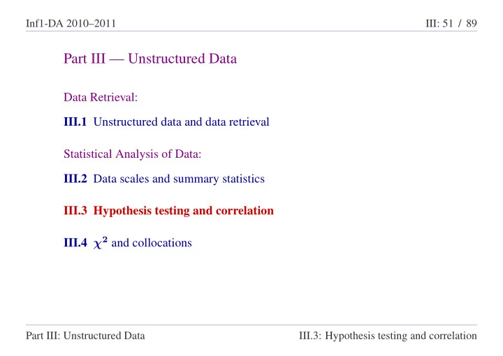
Inf1-DA 2010–2011 III: 51 / 89

Part III — Unstructured Data

Data Retrieval: III.1 Unstructured data and data retrieval Statistical Analysis of Data: III.2 Data scales and summary statistics III.3 Hypothesis testing and correlation III.4 χ2 and collocations

Part III: Unstructured Data III.3: Hypothesis testing and correlation

Inf1-DA 2010–2011 III: 52 / 89

Several variables

Often, one wants to relate data in several variables (i.e., multi-dimensional data). For example, the table below tabulates, for eight students (A–H), their weekly time (in hours) spent: studying for Data & Analysis, drinking and

• eating. This is juxtaposed with their Data & Analysis exam results.

A B C D E F G H Study 0.5 1 1.4 1.2 2.2 2.4 3 3.5 Drinking 25 20 22 10 14 5 2 4 Eating 4 7 4.5 5 8 3.5 6 5 Exam 16 35 42 45 60 72 85 95 Thus, we have four variables: study, drinking, eating and exam. (This is four-dimensional data.)

Part III: Unstructured Data III.3: Hypothesis testing and correlation

Inf1-DA 2010–2011 III: 53 / 89

Correlation

We can ask if there is any relationship between the values taken by two variables. If there is no relationship, then the variables are said to be independent. If there is a relationship, then the variables are said to be correlated. Caution: A correlation does not imply a causal relationship between one variable and another. For example, there is a positive correlation between incidences of lung cancer and time spent watching television, but neither causes the other. However, in cases in which there is a causal relationship between two variables, then there often will be an associated correlation between the variables.

Part III: Unstructured Data III.3: Hypothesis testing and correlation

Inf1-DA 2010–2011 III: 54 / 89

Visualising correlations

One way of discovering correlations is to visualise the data. A simple visual guide is to draw a scatter plot using one variable for the x-axis and one for the y-axis. Example: In the example data on Slide III: 52, is there a correlation between study hours and exam results? What about between drinking hours and exam results? What about eating and exam results?

Part III: Unstructured Data III.3: Hypothesis testing and correlation

Inf1-DA 2010–2011 III: 55 / 89

Studying vs. exam results

This looks like a positive correlation.

Part III: Unstructured Data III.3: Hypothesis testing and correlation

Inf1-DA 2010–2011 III: 56 / 89

Drinking vs. exam results

This looks like a negative correlation.

Part III: Unstructured Data III.3: Hypothesis testing and correlation

Inf1-DA 2010–2011 III: 57 / 89

Eating vs. exam results

There is no obvious correlation.

Part III: Unstructured Data III.3: Hypothesis testing and correlation

Inf1-DA 2010–2011 III: 58 / 89

Statistical hypothesis testing

The last three slides use data visualisation as a tool for postulating hypotheses about data. One might also postulate hypotheses for other reasons, e.g.: intuition that a hypothesis may be true; a perceived analogy with another situation in which a similar hypothesis is known to be valid; existence of a theoretical model that makes a prediction; etc. Statistics provides the tools needed to corroborate or refute such hypotheses with scientific rigour: statistical tests.

Part III: Unstructured Data III.3: Hypothesis testing and correlation

Inf1-DA 2010–2011 III: 59 / 89

The general form of a statistical test

One applies an appropriately chosen statistical test to the data and calculates the result R. Statistical tests are usually based on a null hypothesis that there is nothing

• ut of the ordinary about the data.

The result R of the test has an associated probability value p. The value p represents the probability that we would obtain a result similar to R if the null hypothesis were true. N.B., p is not the probability that the null hypothesis is true. This is not a quantifiable value.

Part III: Unstructured Data III.3: Hypothesis testing and correlation

Inf1-DA 2010–2011 III: 60 / 89

The general form of a statistical test (continued)

The value p represents the probability that we would obtain a result similar to R if the null hypothesis were true. If the value of p is significantly small then we conclude that the null hypothesis is a poor explanation for our data. Thus we reject the null hypothesis, and replace it with a better explanation for our data. Standard significance thresholds are to require p < 0.05 (i.e., there is a less than 1/20 chance that we would have obtained our test result were the null hypothesis true) or, better, p < 0.01 (i.e., there is a less than 1/100 chance)

Part III: Unstructured Data III.3: Hypothesis testing and correlation

Inf1-DA 2010–2011 III: 61 / 89

Correlation coefficient

The correlation coefficient is a statistical measure of how closely the data values x1, . . . , xN are correlated with y1, . . . , yN. Let µx and σx be the mean and standard deviation of the x values. Let µy and σy be the mean and standard deviation of the y values. The correlation coefficient ρx,y is defined by: ρx,y = N

i=1(xi − µx)(yi − µy)

Nσxσy If ρx,y is positive this suggests x, y are positively correlated. If ρx,y is negative this suggests x, y are negatively correlated. If ρx,y is close to 0 this suggests there is no correlation.

Part III: Unstructured Data III.3: Hypothesis testing and correlation

Inf1-DA 2010–2011 III: 62 / 89

Correlation coefficient as a statistical test

In a test for correlation between two variables x, y (e.g., exam result and study hours), we are looking for a correlation and a direction for the correlation (either negative or positive) between the variables. The null hypothesis is that there is no correlation. We calculate the correlation coefficient ρx,y. We then look up significance in a critical values table for the correlation

• coefficient. Such tables can be found in statistics books (and on the Web).

This gives us the associated probability value p. The value of p tells us whether we have significant grounds for rejecting the null hypothesis, in which case our better explanation is that there is a correlation.

Part III: Unstructured Data III.3: Hypothesis testing and correlation

Inf1-DA 2010–2011 III: 63 / 89

Critical values table for the correlation coefficient

The table has rows for N values and columns for p values. N p = 0.1 p = 0.05 p = 0.01 p = 0.001 7 0.669 0.754 0.875 0.951 8 0.621 0.707 0.834 0.925 9 0.582 0.666 0.798 0.898 The table shows that for N = 8 a value of |ρx,y| > 0.834 has probability p < 0.01 of occurring (that is less than a 1/100 chance of occurring) if the null hypothesis is true. Similarly, for N = 8 a value of |ρx,y| > 0.925 has probability p < 0.001 of occurring (that is less than a 1/1000 chance of occurring) if the null hypothesis is true.

Part III: Unstructured Data III.3: Hypothesis testing and correlation

Inf1-DA 2010–2011 III: 64 / 89

Studying vs. exam results

We use the data from III: 52 (see also III: 55), with the study values for x1, . . . , xN, and the exam values for y1, . . . , yN, where N = 8. The relevant statistics are: µx = 1.9 σx = 0.981 µy = 56.25 σy = 24.979 ρx,y = 0.985 Our value of 0.985 is (much) higher than the critical value 0.925. Thus we reject the null hypothesis with very high confidence (p < 0.001) and conclude that there is a correlation. It is a positive correlation since ρx,y is positive not negative.

Part III: Unstructured Data III.3: Hypothesis testing and correlation

Inf1-DA 2010–2011 III: 65 / 89

Drinking vs. exam results

We now use the drinking values from III: 52 (see also III: 56) as the values for x1, . . . , x8. (The y values are unchanged.) The new statistics are: µx = 12.75 σx = 8.288 ρx,y = −0.914 Since | − 0.914| = 0.914 > 0.834, we can reject the null hypothesis with confidence (p < 0.01). This result is still significant though less so than the previous. This time, the value −0.914 of ρx,y is negative so we conclude that there is a negative correlation

Part III: Unstructured Data III.3: Hypothesis testing and correlation

Inf1-DA 2010–2011 III: 66 / 89

Estimating correlation from a sample

As on slides III: 47–48, assume samples x1, . . . , xn and y1, . . . , yn from a population of size N where n < < N. Let m

x and m y be the estimates of the means of the x and y values (V: 47)

Let sx and sy be the estimates of the standard deviations (V: 48) The best estimate rx,y of the correlation coefficient is given by: rx,y = n

i=1(xi − mx)(yi − my)

(n − 1)sxsy The correlation coefficient is sometimes called Pearson’s correlation coefficient, particularly when it is estimated from a sample using the formula above.

Part III: Unstructured Data III.3: Hypothesis testing and correlation

Inf1-DA 2010–2011 III: 67 / 89

Correlation coefficient — subtleties

The correlation coefficient measures how close a scatter plot of x, y values is to a straight line. Nonetheless, a high correlation does not mean that the relationship between x, y is linear. It just means it can be reasonably closely approximated by a linear relationship. Critical value tables for the correlation coefficient are often given with rows indexed by degrees of freedom rather than by N. For the correlation coefficient, the number of degrees of freedom is N − 2, so it is easy to translate such a table into the form given here. (The notion of degree of freedom, in the case of correlation, is too advanced a concept for D&A.) Also, critical value tables often have two classifications: one for one-tailed tests and one for two-tailed tests. Here, we are applying a two-tailed test: we consider both positive and negative values as significant. In a one-tailed test, we would be interested in just one of these possibilities.

Part III: Unstructured Data III.3: Hypothesis testing and correlation