Generative models for social network data Kevin S. Xu (University - - PowerPoint PPT Presentation

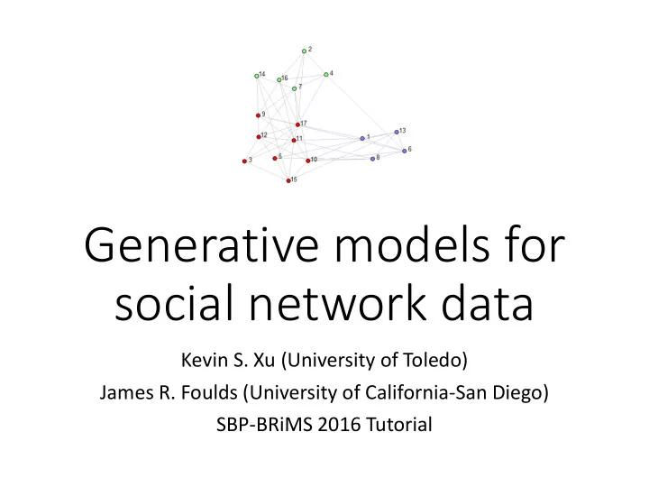
Generative models for social network data

Kevin S. Xu (University of Toledo) James R. Foulds (University of California-San Diego) SBP-BRiMS 2016 Tutorial

About Us

Kevin S. Xu

• Assistant professor at

University of Toledo

• 3 years research

experience in industry

• Research interests:
• Machine learning
• Network science
• Physiological data

analysis James R. Foulds

• Postdoctoral scholar at

UCSD

• Research interests:
• Bayesian modeling
• Social networks
• Text
• Latent variable models

Outline

• Mathematical representations of social networks

and generative models

• Introduction to generative approach
• Connections to sociological principles
• Fitting generative social network models to data
• Example application scenarios
• Model selection and evaluation
• Recent developments in generative social network

models

• Dynamic social network models

Social networks today

Social network analysis: an interdisciplinary endeavor

• Sociologists have been

studying social networks for decades!

• First known empirical

study of social networks: Jacob Moreno in 1930s

• Moreno called them

sociograms

• Recent interest in social

network analysis (SNA) from physics, EECS, statistics, and many other disciplines

Social networks as graphs

• A social network can be represented by a graph 𝐻 = 𝑊, 𝐹
• 𝑊: vertices, nodes, or actors typically representing people
• 𝐹: edges, links, or ties denoting relationships between nodes
• Directed graphs used to represent asymmetric relationships
• Graphs have no natural representation in a geometric space
• Two identical graphs drawn differently
• Moral: visualization provides very limited analysis ability
• How do we model and analyze social network data?

Matrix representation of social networks

• Represent graph by 𝑜 × 𝑜 adjacency matrix or

sociomatrix 𝐙

• 𝑧𝑗𝑘 = 1 if there is an edge between nodes 𝑗 and 𝑘
• 𝑧𝑗𝑘 = 0 otherwise
• Easily extended to directed and weighted graphs

𝐙 = 1 1 1 1 1 1 1 1 1 1 1 1 1 1

Exchangeability of nodes

• Nodes are typically assumed to be (statistically)

exchangeable by symmetry

• Row and column permutations to adjacency matrix

do not change graph

• Needs to be incorporated into social network models

Sociological principles related to edge formation

• Homophily or assortative mixing
• Tendency for individuals to bond with similar others
• Assortative mixing by age, gender, social class,
• rganizational role, node degree, etc.
• Results in transitivity (triangles) in social networks
• “My friend of my friend is my friend”
• Equivalence of nodes
• Two nodes are structurally equivalent if their relations to

all other nodes are identical

• Approximate equivalence recorded by similarity measure
• Two nodes are regularly equivalent if their neighbors are

similar (not necessarily common neighbors)

Brief history of social network models

• Early 1900s – sociology and social psychology precursors to SNA (Georg Simmel)
• 1930s – Graphical depictions of social networks: sociograms (Jacob Moreno)
• 1960s – Small world / 6-degrees of separation experiment (Stanley Milgram)
• 1970s – Mathematical models of social networks (Erdos-Renyi-Gilbert)
• 1980s – Statistical models (Holland and Leinhardt, Frank and Strauss)
• 1990s – Statistical physicists weigh in: preferential attachment, small world

models, power-law degree distributions (Barabasi et al.)

• 2000s – Today – Machine learning approaches, latent variable models

Generative models for social networks

• A generative model is one that can simulate

new networks

• Two distinct schools of thought:
• Probability models (non-statistical)
• Typically simple, 1-2 parameters, not learned from data
• Can be studied analytically
• Statistical models
• More parameters, latent variables
• Learned from data via statistical techniques

Probability and Inference

12

Data generating process Observed data Probability Inference

Figure based on one by Larry Wasserman, "All of Statistics"

Mathematics/physics: Erdős-Rényi, preferential attachment,… Statistics/machine learning: ERGMs, latent variable models…

13

Probability models for networks (non-statistical)

Erdős-Rényi model

• There are two variants of this model
• The model is a probability distribution over

graphs with a fixed number of edges.

• It posits that all graphs on N nodes with E edges are

equally likely

Erdős-Rényi model

• The model posits that each edge is “on”

with probability p

• Probability of adjacency matrix

Erdős-Rényi model

• Adjacency matrix likelihood:
• Number of edges is binomial.
• For large N, this is well approximated by a Poisson

Preferential attachment models

• The Erdős-Rényi model assumes nodes typically

have about the same degree (# edges)

• Many real networks have a degree distribution

following a power law (possibly controversial?)

• Preferential attachment is a variant on the G(N,p)

model to address this (Barabasi and Albert, 1999)

Preferential attachment models

• Initially, no edges, and N0 nodes.
• For each remaining node n
• Add n to the network
• For i =1:m
• Connect n to a random existing node with probability

proportional to its degree ( + smoothing counts),

• A Polya urn process! Rich get richer.

18

Small world models (Watts and Strogatz)

• Start with nodes

connected to K neighbors in a ring

• Randomly rewire

each edge with probability

• Has low average path length (small world

phenomenon, “6-degrees of separation”)

19 Figure due to Arpad Horvath, https://commons.wikimedia.org/wiki/File:Watts_strogatz.svg

20

Statistical network models

Exponential family random graphs (ERGMs)

21

Arbitrary sufficient statistics Covariates (gender, age, …) E.g. “how many males are friends with females”

Exponential family random graphs (ERGMs)

• Pros:
• Powerful, flexible representation
• Can encode complex theories, and do substantive social

science

• Handles covariates
• Mature software tools available,

e.g. ergm package for statnet

22

Exponential family random graphs (ERGMs)

• Cons:
• Usual caveats of undirected models apply
• Computationally intensive, especially learning
• Inference may be intractable, due to partition function
• Model degeneracy can easily happen
• “a seemingly reasonable model can actually be such a bad mis-

specification for an observed dataset as to render the observed data virtually impossible”

• Goodreau (2007)

23

Exponential family random graphs (ERGMs)

• Cons:
• Usual caveats of undirected models apply
• Computationally intensive, especially learning
• Inference may be intractable, due to partition function
• Model degeneracy can easily happen
• “a seemingly reasonable model can actually be such a bad mis-

specification for an observed dataset as to render the observed data virtually impossible”

• Goodreau (2007)

24

Triadic closure

25

If two people have a friend in common, then there is an increased likelihood that they will become friends themselves at some point in the future.

Measuring triadic closure

• Mean clustering co-efficient:

26

+

Simple ERGM for triadic closure leads to model degeneracy

27

Depending on parameters, we could get:

• Graph is empty with probability close to 1
• Graph is full with probability close to 1
• Density, clustering distribution is bimodal, with little

mass on desired density and triad closure MLE may not exist!

Simple ERGM for triadic closure leads to model degeneracy

28

Depending on parameters, we could get:

• Graph is empty with probability close to 1
• Graph is full with probability close to 1
• Density, clustering distribution is bimodal, with little

mass on desired density and triad closure MLE may not exist!

29 Handcock, M. S., Hunter, D. R., Butts, C. T., Goodreau, S. M., & Morris, M. (2008). statnet: Software tools for the representation, visualization, analysis and simulation of network data. Journal of statistical software, 24(1), 1548.

What is the problem?

30

Completes two triangles! If an edge completes more triangles, it becomes overwhelming likely to exist. This propagates to create more triangles …

Solution

• Change the model so that there are diminishing

returns for completing more triangles

• A different natural parameter for each possible number
• f triangles completed by one edge
• Natural parameters parameterized by a lower-

dimensional , e.g. encoding geometrically decreasing weights (curved exponential family)

• Moral of the story: ERGMS are powerful, but

require care and expertise to perform well

31

Latent variable models for social networks

• Model where observed variables are dependent on

a set of unobserved or latent variables

• Observed variables assumed to be conditionally

independent given latent variables

• Why latent variable models?
• Adjacency matrix 𝐙 is invariant to row and column

permutations

• Aldous-Hoover theorem implies existence of a latent

variable model of form for iid latent variables and some function

Latent variable models for social networks

• Latent variable models allow for heterogeneity of

nodes in social networks

• Each node (actor) has a latent variable 𝐴𝑗
• Probability of forming edge between two nodes is

independent of all other node pairs given values of latent variables 𝑞 𝐙 𝐚, 𝜄 = 𝑞 𝑧𝑗𝑘 𝐴𝑗, 𝐴𝑘, 𝜄

𝑗≠𝑘

• Ideally latent variables should provide an interpretable

representation

(Continuous) latent space model

• Motivation: homophily or assortative mixing
• Probability of edge between two nodes increases as

characteristics of the nodes become more similar

• Represent nodes in an unobserved (latent) space of

characteristics or “social space”

• Small distance between 2 nodes in latent space 

high probability of edge between nodes

• Induces transitivity: observation of edges 𝑗, 𝑘 and 𝑘, 𝑙

suggests that 𝑗 and 𝑙 are not too far apart in latent space  more likely to also have an edge

(Continuous) latent space model

• (Continuous) latent space model (LSM) proposed

by Hoff et al. (2002)

• Each node has a latent position 𝐴𝑗 ∈ ℝ𝑒
• Probabilities of forming edges depend on distances

between latent positions

• Define pairwise affinities 𝜔𝑗𝑘 = 𝜄 − 𝐴𝑗 − 𝐴𝑘

2

Latent space model: generative process

• 1. Sample node positions in

latent space

• 2. Compute affinities

between all pairs of nodes

• 3. Sample edges between all

pairs of nodes

Figure due to P. D. Hoff, Modeling homophily and stochastic equivalence in symmetric relational data, NIPS 2008

Advantages and disadvantages of latent space model

• Advantages of latent space model
• Visual and interpretable spatial representation of

network

• Models homophily (assortative mixing) well via

transitivity

• Disadvantages of latent space model
• 2-D latent space representation often may not offer

enough degrees of freedom

• Cannot model disassortative mixing (people preferring

to associate with people with different characteristics)

Stochastic block model (SBM)

• First formalized by Holland et al.

(1983)

• Also known as multi-class Erdős-

Rényi model

• Each node has categorical latent

variable 𝑨𝑗 ∈ 1, … , 𝐿 denoting its class or group

• Probabilities of forming edges

depend on class memberships of nodes (𝐿 × 𝐿 matrix W)

• Groups often interpreted as

functional roles in social networks

Stochastic equivalence and block models

• Stochastic equivalence:

generalization of structural equivalence

• Group members have

identical probabilities of forming edges to members

• ther groups
• Can model both assortative and

disassortative mixing

Figure due to P. D. Hoff, Modeling homophily and stochastic equivalence in symmetric relational data, NIPS 2008

Stochastic equivalence vs community detection

Original graph Blockmodel

Figure due to Goldenberg et al. (2009) - Survey of Statistical Network Models, Foundations and Trends

Stochastically equivalent, but are not densely connected

Stochastic blockmodel Latent representation

UCSD UCI UCLA Alice 1 Bob 1 Claire 1

Alice Bob Claire

Reordering the matrix to show the inferred block structure

Kemp, Charles, et al. "Learning systems of concepts with an infinite relational model." AAAI. Vol. 3. 2006.

Model structure

Kemp, Charles, et al. "Learning systems of concepts with an infinite relational model." AAAI. Vol. 3. 2006.

Latent groups Z Interaction matrix W (probability of an edge from block k to block k’)

Stochastic block model generative process

44

Stochastic block model Latent representation

Running Dancing Fishing Alice 1 Bob 1 Claire 1

Alice Bob Claire Nodes assigned to only

• ne latent group.

Not always an appropriate assumption

Mixed membership stochastic blockmodel (MMSB)

Running Dancing Fishing Alice 0.4 0.4 0.2 Bob 0.5 0.5 Claire 0.1 0.9

Alice Bob Claire Nodes represented by distributions

• ver latent groups (roles)

Airoldi et al., (2008)

Mixed membership stochastic blockmodel (MMSB)

Airoldi et al., (2008)

Latent feature models

Cycling Fishing Running Waltz Running Tango Salsa Alice Bob Claire Mixed membership implies a kind of “conservation of (probability) mass” constraint: If you like cycling more, you must like running less, to sum to one

Miller, Griffiths, Jordan (2009)

Latent feature models

Mixed membership implies a kind of “conservation of (probability) mass” constraint: If you like cycling more, you must like running less, to sum to one

Miller, Griffiths, Jordan (2009)

Cycling Fishing Running Waltz Running Tango Salsa Alice Bob Claire

Latent feature models

Mixed membership implies a kind of “conservation of (probability) mass” constraint: If you like cycling more, you must like running less, to sum to one

Miller, Griffiths, Jordan (2009)

Cycling Fishing Running Waltz Running Tango Salsa Alice Bob Claire

Latent feature models

Miller, Griffiths, Jordan (2009)

Cycling Fishing Running Waltz Running Tango Salsa

Cycling Fishing Running Tango Salsa Waltz Alice Bob Claire

Z =

Alice Bob Claire Nodes represented by binary vector of latent features

Latent feature models

• Latent Feature Relational Model LFRM

(Miller, Griffiths, Jordan, 2009) likelihood model:

• “If I have feature k, and you have feature l, add Wkl to the log-odds
• f the probability we interact”
• Can include terms for network density, covariates, popularity,…, as

in the p2 model

52

1

• 

+ 

Outline

• Mathematical representations of social networks

and generative models

• Introduction to generative approach
• Connections to sociological principles
• Fitting generative social network models to data
• Example application scenarios
• Model selection and evaluation
• Recent developments in generative social network

models

• Dynamic social network models

Application 1: Facebook wall posts

• Network of wall posts on Facebook collected by

Viswanath et al. (2009)

• Nodes: Facebook users
• Edges: directed edge from 𝑗 to 𝑘 if 𝑗 posts on 𝑘’s

Facebook wall

• What model should we use?
• (Continuous) latent space and latent feature models do

not handle directed graphs in a straightforward manner

• Wall posts might not be transitive, unlike friendships
• Stochastic block model might not be a bad choice

as a starting point

Model structure

Kemp, Charles, et al. "Learning systems of concepts with an infinite relational model." AAAI. Vol. 3. 2006.

Latent groups Z Interaction matrix W (probability of an edge from block k to block k’)

Fitting stochastic block model

• A priori block model: assume that class (role) of

each node is given by some other variable

• Only need to estimate 𝑋𝑙𝑙′: probability that node in

class 𝑙 connects to node in class 𝑙′ for all 𝑙, 𝑙′

• Likelihood given by
• Maximum-likelihood estimate (MLE) given by

Number of actual edges in block 𝑙, 𝑙′ Number of possible edges in block 𝑙, 𝑙′

Estimating latent classes

• Latent classes (roles) are unknown in this data set
• First estimate latent classes 𝐚 then use MLE for 𝐗
• MLE over latent classes is intractable!
• ~𝐿𝑂 possible latent class vectors
• Spectral clustering techniques have been shown to

accurately estimate latent classes

• Use singular vectors of (possibly transformed) adjacency

matrix to estimate classes

• Many variants with differing theoretical guarantees

Spectral clustering for directed SBMs

• 1. Compute singular value decomposition

𝑍 = 𝑉Σ𝑊𝑈

• 2. Retain only first 𝐿 columns of 𝑉, 𝑊 and first 𝐿

rows and columns of Σ

• 3. Define coordinate-scaled singular vector matrix

𝑎 = 𝑉Σ1/2 𝑊Σ1/2

• 4. Run k-means clustering on rows of 𝑎

to return estimate 𝑎

• f latent classes

Scales to networks with thousands of nodes!

Demo of SBM on Facebook wall post network

Application 2: social network of bottlenose dolphin interactions

• Data collected by marine biologists observing

interactions between 62 bottlenose dolphins

• Introduced to network science community by Lusseau

and Newman (2004)

• Nodes: dolphins
• Edges: undirected relations denoting frequent

interactions between dolphins

• What model should we use?
• Social interactions here are in a group setting so lots of

transitivity may be expected

• Interactions associated by physical proximity
• Use latent space model to estimate latent positions

(Continuous) latent space model

• (Continuous) latent space model (LSM) proposed

by Hoff et al. (2002)

• Each node has a latent position 𝐴𝑗 ∈ ℝ𝑒
• Probabilities of forming edges depend on distances

between latent positions

• Define pairwise affinities 𝜔𝑗𝑘 = 𝜄 − 𝐴𝑗 − 𝐴𝑘

2

𝑞 𝑍 𝑎, 𝜄 = 𝑓𝑧𝑗𝑘𝜔𝑗𝑘 1 + 𝑓𝜔𝑗𝑘

𝑗≠𝑘

Estimation for latent space model

• Maximum-likelihood estimation
• Log-likelihood is concave in terms of pairwise distance

matrix 𝐸 but not in latent positions 𝑎

• First find MLE in terms of 𝐸 then use multi-dimensional

scaling (MDS) to get initialization for 𝑎

• Faster approach: replace 𝐸 with shortest path distances

in graph then use MDS

• Use non-linear optimization to find MLE for 𝑎
• Latent space dimension often set to 2 to allow

visualization using scatter plot Scales to ~1000 nodes

Demo of latent space model on dolphin network

Bayesian inference

• As a Bayesian, all you have to do is write down your

prior beliefs, write down your likelihood, and apply Bayes ‘ rule,

64

Elements of Bayesian Inference

65

Posterior Likelihood Marginal likelihood (a.k.a. model evidence) Prior is a normalization constant that does not depend on the value of θ. It is the probability of the data under the model, marginalizing over all possible θ’s.

The full posterior distribution can be very useful

66

The mode (MAP estimate) is unrepresentative of the distribution

MAP estimate can result in

• verfitting

67

Markov chain Monte Carlo

• Goal: approximate/summarize a distribution, e.g.

the posterior, with a set of samples

• Idea: use a Markov chain to simulate the

distribution and draw samples

68

Gibbs sampling

• Sampling from a complicated distribution, such as a

Bayesian posterior, can be hard.

• Often, sampling one variable at a time, given all the
• thers, is much easier.
• Graphical models:

Graph structure gives us Markov blanket

69

Gibbs sampling

• Update variables one at a time by drawing from

their conditional distributions

• In each iteration, sweep through and update all of

the variables, in any order.

70

Gibbs sampling

71

Gibbs sampling

72

Gibbs sampling

73

Gibbs sampling

74

Gibbs sampling

75

Gibbs sampling

76

Gibbs sampling

77

Gibbs sampling for SBM

Variational inference

• Key idea:
• Approximate distribution of interest p(z) with another

distribution q(z)

• Make q(z) tractable to work with
• Solve an optimization problem to make q(z) as similar to

p(z) as possible, e.g. in KL-divergence

79

Variational inference

80

p q

Variational inference

81

p q

Variational inference

82

p q

83

Blows up if p is small and q isn’t. Under-estimates the support Blows up if q is small and p isn’t. Over-estimates the support Reverse KL Forwards KL

Figures due to Kevin Murphy (2012). Machine Learning: A Probabilistic Perspective

KL-divergence as an objective function for variational inference

• Minimizing the KL is equivalent to maximizing

84

Fit the data well Be flat

KL-divergence as an objective function for variational inference

• Minimizing the KL is equivalent to maximizing

85

Fit the data well Be flat

KL-divergence as an objective function for variational inference

• Minimizing the KL is equivalent to maximizing

86

Fit the data well Be flat

KL-divergence as an objective function for variational inference

• Minimizing the KL is equivalent to maximizing

87

Fit the data well Be flat

Mean field variational inference

• We still need to compute expectations over z
• However, we have gained the option to restrict q(z)

to make these expectations tractable.

• The mean field approach uses a fully factorized q(z)

88

The entropy term decomposes nicely:

Mean field algorithm

• Until converged
• For each factor i
• Select variational parameters such that
• Each update monotonically improves the ELBO so

the algorithm must converge

89

Deriving mean field updates for your model

• Write down the mean field equation explicitly,
• Simplify and apply the expectation.
• Manipulate it until you can recognize it as a log-pdf
• f a known distribution (hopefully).
• Reinstate the normalizing constant.

90

Mean field vs Gibbs sampling

• Both mean field and Gibbs sampling iteratively

update one variable given the rest

• Mean field stores an entire distribution for each

variable, while Gibbs sampling draws from one.

91

Pros and cons vs Gibbs sampling

• Pros:
• Deterministic algorithm, typically converges faster
• Stores an analytic representation of the distribution, not just

samples

• Non-approximate parallel algorithms
• Stochastic algorithms can scale to very large data sets
• No issues with checking convergence
• Cons:
• Will never converge to the true distribution,

unlike Gibbs sampling

• Dense representation can mean more communication for parallel

algorithms

• Harder to derive update equations

92

Variational inference algorithm for MMSB (Variational EM)

• Compute maximum likelihood estimates for interaction

parameters Wkk’

• Assume fully factorized variational distribution for

mixed membership vectors, cluster assignments

• Until converged
• For each node
• Compute variational discrete distribution over it’s latent

zp->q and zq->p assignments

• Compute variational Dirichlet distribution over its mixed

membership distribution

• Maximum likelihood update for W

Application of MMSB to Sampson’s Monastery

• Sampson (1968) studied

friendship relationships between novice monks

• Identified several factions
• Blockmodel appropriate?
• Conflicts occurred
• Two monks expelled
• Others left

Airoldi, E. M., Blei, D. M., Fienberg, S. E., & Xing, E. P. (2009). Mixed membership stochastic blockmodels. In Advances in Neural Information Processing Systems (pp. 33-40).

Application of MMSB to Sampson’s Monastery

Airoldi, E. M., Blei, D. M., Fienberg, S. E., & Xing, E. P. (2009). Mixed membership stochastic blockmodels. In Advances in Neural Information Processing Systems (pp. 33-40).

Estimated blockmodel

Application of MMSB to Sampson’s Monastery

Airoldi, E. M., Blei, D. M., Fienberg, S. E., & Xing, E. P. (2009). Mixed membership stochastic blockmodels. In Advances in Neural Information Processing Systems (pp. 33-40).

Estimated blockmodel Least coherent

Application of MMSB to Sampson’s Monastery

Airoldi, E. M., Blei, D. M., Fienberg, S. E., & Xing, E. P. (2009). Mixed membership stochastic blockmodels. In Advances in Neural Information Processing Systems (pp. 33-40).

Estimated Mixed membership vectors (posterior mean)

Application of MMSB to Sampson’s Monastery

Airoldi, E. M., Blei, D. M., Fienberg, S. E., & Xing, E. P. (2009). Mixed membership stochastic blockmodels. In Advances in Neural Information Processing Systems (pp. 33-40).

Estimated Mixed membership vectors (posterior mean) Expelled

Application of MMSB to Sampson’s Monastery

Airoldi, E. M., Blei, D. M., Fienberg, S. E., & Xing, E. P. (2009). Mixed membership stochastic blockmodels. In Advances in Neural Information Processing Systems (pp. 33-40).

Estimated Mixed membership vectors (posterior mean) Wavering not captured

Application of MMSB to Sampson’s Monastery

Airoldi, E. M., Blei, D. M., Fienberg, S. E., & Xing, E. P. (2009). Mixed membership stochastic blockmodels. In Advances in Neural Information Processing Systems (pp. 33-40).

Original network (whom do you like?) Summary of network (use π‘s)

Application of MMSB to Sampson’s Monastery

Airoldi, E. M., Blei, D. M., Fienberg, S. E., & Xing, E. P. (2009). Mixed membership stochastic blockmodels. In Advances in Neural Information Processing Systems (pp. 33-40).

Original network (whom do you like?) Denoise network (use z’s)

Scaling up Bayesian inference to large networks

• Two key strategies: parallel/distributed, and stochastic

algorithms

• Parallel/distributed algorithms
• Compute VB or MCMC updates in parallel
• Communication overhead may be lower for MCMC
• Not well understood for MCMC, but works in practice
• Stochastic algorithms
• Stochastic variational inference
• estimate updates based on subsamples. MMSB: Gopalan et al. (2012)
• A related subsampling trick for MCMC in latent space models (Raftery et

al., 2012)

• Other general stochastic MCMC algorithms:
• Stochastic gradient Langevin dynamics (Welling and Teh, 2011), Austerity MCMC

(Korattika et al., 2014)

Evaluation of unsupervised models

• Quantitative evaluation
• Measurable, quantifiable performance metrics
• Qualitative evaluation
• Exploratory data analysis (EDA) using the model
• Human evaluation, user studies,…

103

Evaluation of unsupervised models

• Intrinsic evaluation
• Measure inherently good properties of the model
• Fit to the data (e.g. link prediction), interpretability,…
• Extrinsic evaluation
• Study usefulness of model for external tasks
• Classification, retrieval, part of speech tagging,…

104

Extrinsic evaluation: What will you use your model for?

• If you have a downstream task in mind, you should

probably evaluate based on it!

• Even if you don’t, you could contrive one for

evaluation purposes

• E.g. use latent representations for:
• Classification, regression, retrieval, ranking…

105

Posterior predictive checks

• Sampling data from the posterior predictive distribution

allows us to “look into the mind of the model” – G. Hinton

106

“This use of the word mind is not intended to be metaphorical. We believe that a mental state is the state of a hypothetical, external world in which a high-level internal representation would constitute veridical perception. That hypothetical world is what the figure shows.” Geoff Hinton et al. (2006), A Fast Learning Algorithm for Deep Belief Nets.

Posterior predictive checks

• Does data drawn from the model differ from the
• bserved data, in ways that we care about?
• PPC:
• Define a discrepancy function (a.k.a. test statistic) T(X).
• Like a test statistic for a p-value. How extreme is my data set?
• Simulate new data X(rep) from the posterior predictive
• Use MCMC to sample parameters from posterior, then simulate data
• Compute T(X(rep)) and T(X), compare. Repeat, to estimate:

107

Outline

• Mathematical representations of social networks

and generative models

• Introduction to generative approach
• Connections to sociological principles
• Fitting generative social network models to data
• Example application scenarios
• Model selection and evaluation
• Recent developments in generative social network

models

• Dynamic social network models

Dynamic social network

• Relations between people may change over time
• Need to generalize social network models to

account for dynamics

Dynamic social network (Nordlie, 1958; Newcomb, 1961)

Dynamic Relational Infinite Feature Model (DRIFT)

• J. R. Foulds, A. Asuncion, C. DuBois, C. T. Butts, P. Smyth.

A dynamic relational infinite feature model for longitudinal social networks. AISTATS 2011

• Models networks as they over time, by way of

changing latent features

Cycling Fishing Running Waltz Running Tango Salsa Alice Bob Claire

Dynamic Relational Infinite Feature Model (DRIFT)

• Models networks as they over time, by way of

changing latent features

Cycling Fishing Running Waltz Running Tango Salsa Alice Bob Claire

• J. R. Foulds, A. Asuncion, C. DuBois, C. T. Butts, P. Smyth.

A dynamic relational infinite feature model for longitudinal social networks. AISTATS 2011

Dynamic Relational Infinite Feature Model (DRIFT)

• Models networks as they over time, by way of

changing latent features

Cycling Fishing Running Waltz Running Tango Salsa Alice Bob Claire

• J. R. Foulds, A. Asuncion, C. DuBois, C. T. Butts, P. Smyth.

A dynamic relational infinite feature model for longitudinal social networks. AISTATS 2011

Dynamic Relational Infinite Feature Model (DRIFT)

• Models networks as they over time, by way of

changing latent features

Cycling Fishing Running Waltz Running Tango Salsa Fishing Alice Bob Claire

• J. R. Foulds, A. Asuncion, C. DuBois, C. T. Butts, P. Smyth.

A dynamic relational infinite feature model for longitudinal social networks. AISTATS 2011

Dynamic Relational Infinite Feature Model (DRIFT)

• Models networks as they over time, by way of

changing latent features

Cycling Fishing Running Waltz Running Tango Salsa Fishing Alice Bob Claire

• J. R. Foulds, A. Asuncion, C. DuBois, C. T. Butts, P. Smyth.

A dynamic relational infinite feature model for longitudinal social networks. AISTATS 2011

Dynamic Relational Infinite Feature Model (DRIFT)

• Models networks as they over time, by way of

changing latent features

• HMM dynamics for each actor/feature (factorial HMM)
• J. R. Foulds, A. Asuncion, C. DuBois, C. T. Butts, P. Smyth.

A dynamic relational infinite feature model for longitudinal social networks. AISTATS 2011

Bayesian Inference for DRIFT

• Markov chain Monte Carlo inference
• Blocked Gibbs sampler
• Forward filtering, backward sampling to jointly sample

each actor's feature chains

• “Slice sampling” trick with the stick-breaking

construction of the IBP to adaptively truncate the number of features but still perform exact inference

• Metropolis-Hastings updates for W's
• J. R. Foulds, A. Asuncion, C. DuBois, C. T. Butts, P. Smyth.

A dynamic relational infinite feature model for longitudinal social networks. AISTATS 2011

Synthetic Data: Inference on Z’s

• J. R. Foulds, A. Asuncion, C. DuBois, C. T. Butts, P. Smyth.

A dynamic relational infinite feature model for longitudinal social networks. AISTATS 2011

Synthetic Data: Predicting the Future

• J. R. Foulds, A. Asuncion, C. DuBois, C. T. Butts, P. Smyth.

A dynamic relational infinite feature model for longitudinal social networks. AISTATS 2011

Enron Email Data: Predicting the Future

• J. R. Foulds, A. Asuncion, C. DuBois, C. T. Butts, P. Smyth.

A dynamic relational infinite feature model for longitudinal social networks. AISTATS 2011

Enron Email Data: Predicting the Future

• J. R. Foulds, A. Asuncion, C. DuBois, C. T. Butts, P. Smyth.

A dynamic relational infinite feature model for longitudinal social networks. AISTATS 2011

Enron Email Data: Missing Data Imputation

• J. R. Foulds, A. Asuncion, C. DuBois, C. T. Butts, P. Smyth.

A dynamic relational infinite feature model for longitudinal social networks. AISTATS 2011

Enron Email Data: Edge Probability Over Time

• J. R. Foulds, A. Asuncion, C. DuBois, C. T. Butts, P. Smyth.

A dynamic relational infinite feature model for longitudinal social networks. AISTATS 2011

Quantitative Results

• J. R. Foulds, A. Asuncion, C. DuBois, C. T. Butts, P. Smyth.

A dynamic relational infinite feature model for longitudinal social networks. AISTATS 2011

Hidden Markov dynamic network models

• Most work on dynamic network modeling

assumes hidden Markov structure

– Latent variables and/or parameters follow Markov dynamics – Graph snapshot at each time generated using static network model, e.g. stochastic block model or latent feature model as in DRIFT – Has been used to extend SBMs to dynamic models (Yang et al., 2011; Xu and Hero, 2014)

Beyond hidden Markov networks

• Hidden Markov structure is tractable but not very

realistic assumption in social interaction networks

– Interaction between two people does not influence future interactions

• Proposed model: Allow current graph to depend on

current parameters and previous graph

• Proposed inference procedure does not require MCMC

– Scales to ~ 1000 nodes

Stochastic block transition model

• Generate graph at initial time step using SBM
• Place Markov model on Π𝑢|0, Π𝑢|1
• Main idea: parameterize each block

𝑙, 𝑙′ with two probabilities

– Probability of forming new edge 𝜌𝑙𝑙′

𝑢|0 = Pr 𝑍 𝑗𝑘 𝑢 = 1|𝑍 𝑗𝑘 𝑢−1 = 0

– Probability of existing edge re-

• ccurring

𝜌𝑙𝑙′

𝑢|1 = Pr 𝑍 𝑗𝑘 𝑢 = 1|𝑍 𝑗𝑘 𝑢−1 = 1

Application to Facebook wall posts

• Fit dynamic SBMs to network of Facebook wall posts

– ~ 700 nodes, 9 time steps, 5 classes

• How accurately do hidden Markov SBM and SBTM

replicate edge durations in observed network?

– Simulate networks from both models using estimated parameters – Hidden Markov SBM cannot replicate long-lasting edges in sparse blocks

Behaviors of different classes

• SBTM retains interpretability of SBM at each time step
• Q: Do different classes behave differently in how they form edges?
• A: Only for probability of existing edges re-occurring
• New insight revealed by having separate probabilities in SBTM

Information diffusion in text-based cascades

t=0 t=3.5 t=1 t=2 t=1.5

• Temporal information
• Content information
• Network is latent
• X. He, T. Rekatsinas, J. R. Foulds, L. Getoor, and Y. Liu. HawkesTopic: A joint model for network inference and topic modeling

from text-based cascades. ICML 2015.

HawkesTopic model for text-based cascades

130

Mutual exciting nature: A posting event can trigger future events

Content cascades: The content of a document should be similar

to the document that triggers its publication

• X. He, T. Rekatsinas, J. R. Foulds, L. Getoor, and Y. Liu. HawkesTopic: A joint model for network inference and topic modeling

from text-based cascades. ICML 2015.

Modeling posting times

Mutually exciting nature captured via Multivariate Hawkes Process (MHP) [Liniger 09]. For MHP, intensity process 𝜇𝑤(𝑢) takes the form:

𝜇𝑤 𝑢 = 𝜈𝑤 + 𝐵𝑤𝑓,𝑤𝑔

Δ(𝑢 − 𝑢𝑓) 𝑓:𝑢𝑓<𝑢

𝐵𝑣,𝑥: influence strength from 𝑣 to 𝑤 𝑔

Δ(⋅): probability density function of the delay distribution

Base intensity Influence from previous events

+

Rate =

Clustered Poisson process interpretation

• X. He, T. Rekatsinas, J. R. Foulds, L. Getoor, and Y. Liu. HawkesTopic: A joint model for network inference and topic modeling

from text-based cascades. ICML 2015.

Generating documents

• X. He, T. Rekatsinas, J. R. Foulds, L. Getoor, and Y. Liu. HawkesTopic: A joint model for network inference and topic modeling

from text-based cascades. ICML 2015.

Experiments for HawkesTopic

• X. He, T. Rekatsinas, J. R. Foulds, L. Getoor, and Y. Liu. HawkesTopic: A joint model for network inference and topic modeling

from text-based cascades. ICML 2015.

Results: EventRegistry

• X. He, T. Rekatsinas, J. R. Foulds, L. Getoor, and Y. Liu. HawkesTopic: A joint model for network inference and topic modeling

from text-based cascades. ICML 2015.

Results: EventRegistry

• X. He, T. Rekatsinas, J. R. Foulds, L. Getoor, and Y. Liu. HawkesTopic: A joint model for network inference and topic modeling

from text-based cascades. ICML 2015.

Results: ArXiv

• X. He, T. Rekatsinas, J. R. Foulds, L. Getoor, and Y. Liu. HawkesTopic: A joint model for network inference and topic modeling

from text-based cascades. ICML 2015.

Results: ArXiv

• X. He, T. Rekatsinas, J. R. Foulds, L. Getoor, and Y. Liu. HawkesTopic: A joint model for network inference and topic modeling

from text-based cascades. ICML 2015.

Summary

• Generative models provide a powerful mechanism for

modeling social networks

• Latent variable models offer flexible yet interpretable

models motivated by sociological principles

• Latent space model
• Stochastic block model
• Mixed-membership stochastic block model
• Latent feature model
• Many recent advancements in generative models for

social networks

• Dynamic networks, cascades, joint modeling with text

Thank you!

The giant component

• Depending on the quantity ,

a “giant” connected component may emerge

141

The giant component

• Depending on the quantity ,

a “giant” connected component may emerge

142

The giant component

• Depending on the quantity ,

a “giant” connected component may emerge

143