Last time 6.891 Computer Vision and Applications Interesting - PDF document
Last time 6.891 Computer Vision and Applications Interesting points, correspondence, affine patch tracking Prof. Trevor. Darrell Scale and rotation invariant descriptors [Lowe] Lecture 7: Features and Geometry Affine invariant features
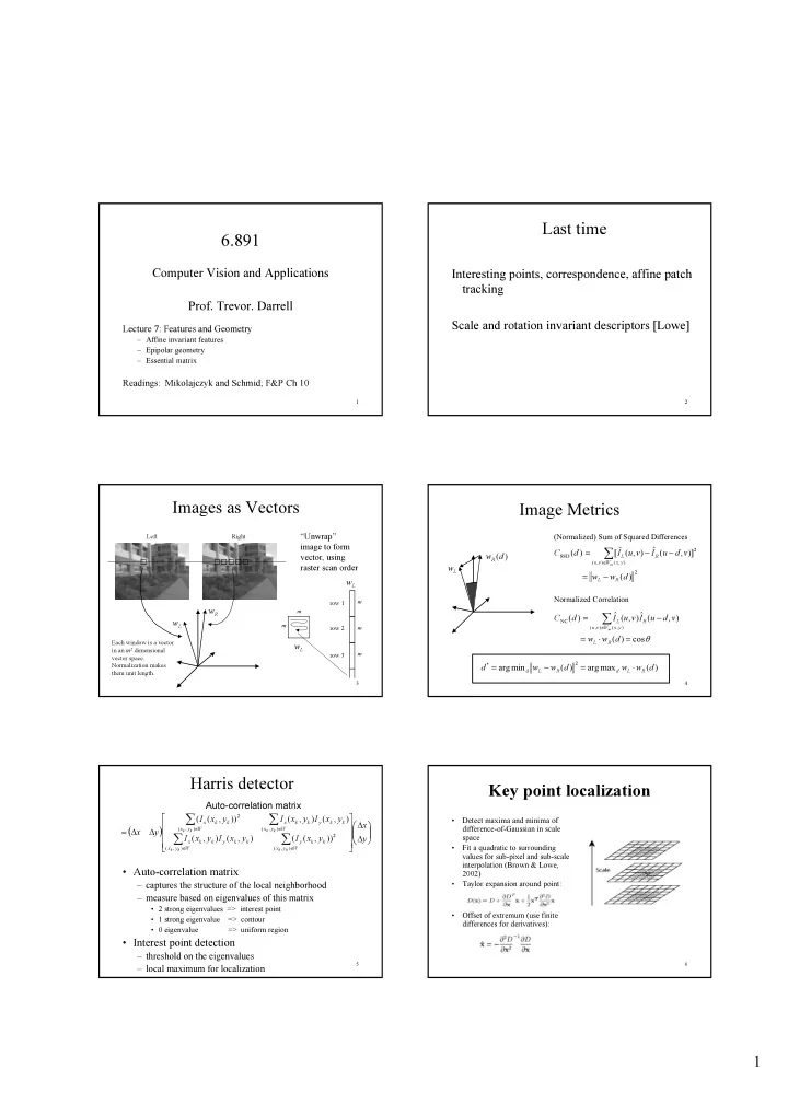
Last time 6.891 Computer Vision and Applications Interesting points, correspondence, affine patch tracking Prof. Trevor. Darrell Scale and rotation invariant descriptors [Lowe] Lecture 7: Features and Geometry – Affine invariant features – Epipolar geometry – Essential matrix Readings: Mikolajczyk and Schmid; F&P Ch 10 1 2 Images as Vectors Image Metrics “Unwrap” Left Right (Normalized) Sum of Squared Differences image to form ˆ ˆ 2 C ( d ) ∑ [ I ( u , v ) I ( u d , v )] = − − w R ( d ) SSD L R vector, using ( u , v ) W ( x , y ) ∈ m raster scan order w L 2 w w ( d ) = − L R w L Normalized Correlation m row 1 w m R ˆ ˆ C ( d ) ∑ I ( u , v ) I ( u d , v ) = − NC L R w L m ( u , v ) W ( x , y ) row 2 m ∈ m w w ( d ) cos θ = ⋅ = Each window is a vector L R w in an m 2 dimensional L row 3 m vector space. 2 * Normalization makes d arg min w w ( d ) arg max w w ( d ) = − = ⋅ d L R d L R them unit length. 3 4 Harris detector Key point localization Auto-correlation matrix 2 ∑ ( I ( x , y )) ∑ I ( x , y ) I ( x , y ) • Detect maxima and minima of x k k x k k y k k ∆ x ( x , y ) W ( x , y ) W difference-of-Gaussian in scale ∈ ∈ = ( ∆ ∆ ) k k k k x y 2 ∆ space ∑ I ( x , y ) I ( x , y ) ∑ ( I ( x , y )) y x k k y k k y k k ( x , y ) ∈ W ( x , y ) ∈ W • Fit a quadratic to surrounding k k k k values for sub-pixel and sub-scale interpolation (Brown & Lowe, • Auto-correlation matrix r u l B 2002) • Taylor expansion around point: – captures the structure of the local neighborhood – measure based on eigenvalues of this matrix • 2 strong eigenvalues => interest point • Offset of extremum (use finite • 1 strong eigenvalue => contour differences for derivatives): • 0 eigenvalue => uniform region • Interest point detection – threshold on the eigenvalues 5 6 – local maximum for localization 1
SIFT vector formation Select canonical orientation • Thresholded image gradients are sampled over 16x16 array of locations in scale space • Create array of orientation histograms • Create histogram of local gradient directions computed • 8 orientations x 4x4 histogram array = 128 dimensions at selected scale • Assign canonical orientation at peak of smoothed histogram • Each key specifies stable 2D coordinates (x, y, scale, orientation) 2 π 0 7 8 Today Affine invariance of interest points Affine Invariant Interest points [Schmid] Cordelia Schmid Evaluation of interest points and descriptors [Schmid] CVPR’03 Tutorial Epipolar geometry and the Essential Matrix 9 10 Scale invariant interest Scale invariant Harris points points • Multi-scale extraction of Harris interest points multi-scale Harris points • Selection of points at characteristic scale in scale space selection of points at the characteristic scale with Laplacian Chacteristic scale : - maximum in scale space Laplacian - scale invariant invariant points + associated regions [Mikolajczyk & 11 12 Schmid’01] 2
Viewpoint changes State of the art • Locally approximated by an affine transformation • Affine invariant regions (Tuytelaars et al.’00) – ellipses fitted to intensity maxima – parallelogram formed by interest points and edges A detected scale invariant region projected region 13 14 State of the art State of the art • Theory for affine invariant neighborhood (Lindeberg’94) • Localization & scale influence affine M = µ ( x , Σ ) M = µ ( x , Σ ) L L L R R R neighhorbood A x → x => affine invariant Harris points (Mikolajczyk & Schmid’02) 1 1 • Iterative estimation of these parameters − − M 2 M 2 x → x x → x L R 1. localization – local maximum of the Harris measure 1 1 2 2 ( M x ) R ( M x ) 2. scale – automatic scale selection with the Laplacian = R R L L 3. affine neighborhood – normalization with second moment matrix Isotropic neighborhoods Repeat estimation until convergence 15 16 related by rotation Affine invariant Harris points Affine invariant Harris points • Iterative estimation of localization, scale, neighborhood • Iterative estimation of localization, scale, neighborhood Initial points Iteration #1 17 18 3
Affine invariant Harris points Affine invariant Harris points • Iterative estimation of localization, scale, neighborhood • Iterative estimation of localization, scale, neighborhood Iteration #2 Iteration #3, #4, ... 19 20 Affine invariant Harris points Affine invariant Harris points • Initialization with multi-scale interest points • Iterative modification of location, scale and neighborhood affine Harris Harris-Laplace Harris-Laplace 21 22 + affine regions Affine invariant neighborhhood Image retrieval affine Harris detector … > 5000 images affine Laplace change in viewing angle detector 23 24 4
Image retrieval Matches … > 5000 images change in viewing angle + scale change 22 correct matches 25 26 3D Recognition Matches 33 correct matches 27 28 3D Recognition Evaluation of interest points and descriptors Cordelia Schmid CVPR’03 Tutorial 3D object modeling and recognition using affine-invariant patches and multi-view spatial constraints, F. Rothganger, S. Lazebnik, C. Schmid, J. Ponce, CVPR 2003 29 30 5
Quantitative evaluation of detectors Introduction • Repeatability rate : percentage of corresponding points • Quantitative evaluation of interest point detectors – points / regions at the same relative location homography => repeatability rate • Quantitative evaluation of descriptors – distinctiveness • Two points are corresponding if => detection rate with respect to false positives 1. The location error is less than 1.5 pixel 2. The intersection error is less than 20% 31 32 Comparison of different detectors Comparison of different detectors repeatability - image rotation repeatability – perspective transformation [Comparing and Evaluating Interest Points, Schmid, Mohr & Bauckhage, ICCV 98] [Comparing and Evaluating Interest Points, Schmid, Mohr & Bauckhage, ICCV 98] 33 34 Harris detector + scale changes Harris detector – adaptation to scale 35 36 6
Evaluation of scale invariant detectors Evaluation of affine invariant detectors repeatability – scale changes repeatability – perspective transformation 0 40 60 70 37 38 Experimental Quantitative evaluation of descriptors evaluation • Evaluation of different local features – SIFT, steerable filters, differential invariants, moment invariants, cross-correlation • Measure : distinctiveness – receiver operating characteristics of detection rate with respect to false positives – detection rate = correct matches / possible matches – false positives = false matches / (database points * query points) [A performance evaluation of local descriptors, Mikolajczyk & Schmid, CVPR’03] 39 40 Scale change (factor 2.5) Viewpoint change (60 degrees) Harris-Laplace DoG Harris-Affine (Harris-Laplace) 41 42 7
Descriptors - conclusion Today • SIFT + steerable perform best Affine Invariant Interest points [Schmid] • Performance of the descriptor independent Evaluation of interest points and descriptors of the detector [Schmid] • Errors due to imprecision in region Epipolar geometry and the Essential Matrix estimation, localization 43 44 Multi-view geometry and 3-D We have 2 eyes, yet we see 3-D! 3-D: The hidden dimension… Using multiple views allows inference of hidden dimension. 45 46 How to see in 3-D (Using geometry…) • Find features • Triangulate & reconstruct depth Multiple views to the rescue! 47 48 8
Multi-view geometry Multi-view geometry Relate Relate • 3-D points 49 50 Multi-view geometry Multi-view geometry Relate Relate • 3-D points • 3-D points • Camera centers • Camera centers • Camera orientation 51 52 Multi-view geometry Multi-view geometry Relate Relate • 3-D points • 3-D points • Camera centers • Camera centers • Camera orientation • Camera orientation • Camera intrinsics • Camera intrinsics 53 54 9
Stereo constraints Stereo constraints Given p in left image, where can p’ be? p ’? p Given p in left image, where can p ’? p corresponding point p’ be? Could be anywhere! Might not be same 55 56 scene! Stereo constraints Epipolar line Given p in left image, where can p’ be? p ’? ? p p DEMO 57 58 Epipolar constraint From geometry to algebra… P p p’ O O’ All epipolar lines contain epipole, the image of other camera center. 59 60 10
Recommend
More recommend
Explore More Topics
Stay informed with curated content and fresh updates.
