6.891 Computer Vision and Applications Prof. Trevor. Darrell - PowerPoint PPT Presentation
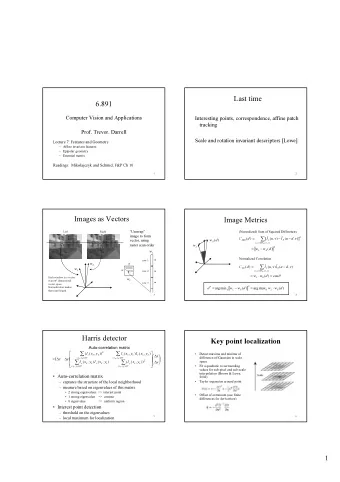
6.891 Computer Vision and Applications Prof. Trevor. Darrell Lecture 16: Tracking Density propagation Linear Dynamic models / Kalman filter Data association Multiple models Readings: F&P Ch 17 1 Syllabus 2 Tracking
6.891 Computer Vision and Applications Prof. Trevor. Darrell Lecture 16: Tracking – Density propagation – Linear Dynamic models / Kalman filter – Data association – Multiple models Readings: F&P Ch 17 1
Syllabus 2
Tracking Applications • Motion capture • Recognition from motion • Surveillance • Targeting 3
Things to consider in tracking What are the • Real world dynamics • Approximate / assumed model • Observation / measurement process 4
Density propogation • Tracking == Inference over time • Much simplification is possible with linear dynamics and Gaussian probability models 5
Outline • Recursive filters • State abstraction • Density propagation • Linear Dynamic models / Kalman filter • Data association • Multiple models 6
Tracking and Recursive estimation • Real-time / interactive imperative. • Task: At each time point, re-compute estimate of position or pose. – At time n, fit model to data using time 0…n – At time n+1, fit model to data using time 0…n+1 • Repeat batch fit every time? 7
Recursive estimation • Decompose estimation problem – part that depends on new observation – part that can be computed from previous history • E.g., running average: a t = α a t-1 + (1- α ) y t • Linear Gaussian models: Kalman Filter • First, general framework… 8
Tracking • Very general model: – We assume there are moving objects, which have an underlying state X – There are measurements Y, some of which are functions of this state – There is a clock • at each tick, the state changes • at each tick, we get a new observation • Examples – object is ball, state is 3D position+velocity, measurements are stereo pairs – object is person, state is body configuration, measurements are frames, clock is in camera (30 fps) 9
Three main issues in tracking 10
Simplifying Assumptions 11
Tracking as induction • Assume data association is done – we’ll talk about this later; a dangerous assumption • Do correction for the 0’th frame • Assume we have corrected estimate for i’th frame – show we can do prediction for i+1, correction for i+1 12
Base case 13
Induction step given 14
Induction step given 15
Linear dynamic models • A linear dynamic model has the form ( ) x i = N D i − 1 x i − 1 ; Σ d i ( ) y i = N M i x i ; Σ m i • This is much, much more general than it looks, and extremely powerful 16
( ) x i = N D i − 1 x i − 1 ; Σ d i Examples ( ) y i = N M i x i ; Σ m i • Drifting points – assume that the new position of the point is the old one, plus noise D = Id 17 cic.nist.gov/lipman/sciviz/images/random3.gif http://www.grunch.net/synergetics/images/random 3.jpg
( ) x i = N D i − 1 x i − 1 ; Σ d i Constant velocity ( ) y i = N M i x i ; Σ m i • We have u i = u i − 1 + ∆ tv i − 1 + ε i v i = v i − 1 + ς i – (the Greek letters denote noise terms) • Stack (u, v) into a single state vector ∆ t u = 1 u + noise v 0 1 v i − 1 i – which is the form we had above 18
velocity position position time measurement,position Constant Velocity Model time 19
( ) x i = N D i − 1 x i − 1 ; Σ d i Constant acceleration ( ) y i = N M i x i ; Σ m i • We have u i = u i − 1 + ∆ tv i − 1 + ε i v i = v i − 1 + ∆ ta i − 1 + ς i a i = a i − 1 + ξ i – (the Greek letters denote noise terms) • Stack (u, v) into a single state vector ∆ t u 1 0 u = ∆ t + noise v 0 1 v a 0 0 1 a i − 1 i – which is the form we had above 20
velocity position position time Constant Acceleration Model 21
( ) x i = N D i − 1 x i − 1 ; Σ d i Periodic motion ( ) y i = N M i x i ; Σ m i Assume we have a point, moving on a line with a periodic movement defined with a differential eq: can be defined as with state defined as stacked position and velocity u=(p, v) 22
( ) x i = N D i − 1 x i − 1 ; Σ d i Periodic motion ( ) y i = N M i x i ; Σ m i Take discrete approximation … .(e.g., forward Euler integration with ∆ t stepsize.) 23
Higher order models • Independence assumption • Velocity and/or acceleration augmented position • Constant velocity model equivalent to – velocity == – acceleration == – could also use , etc. 24
The Kalman Filter • Key ideas: – Linear models interact uniquely well with Gaussian noise - make the prior Gaussian, everything else Gaussian and the calculations are easy – Gaussians are really easy to represent --- once you know the mean and covariance, you’re done 25
Recall the three main issues in tracking (Ignore data association for now) 26
The Kalman Filter 27 [figure from http://www.cs.unc.edu/~welch/kalman/kalmanIntro.html]
The Kalman Filter in 1D • Dynamic Model • Notation Predicted mean Corrected mean 28
The Kalman Filter 29
Prediction for 1D Kalman filter • The new state is obtained by – multiplying old state by known constant – adding zero-mean noise • Therefore, predicted mean for new state is – constant times mean for old state • Old variance is normal random variable – variance is multiplied by square of constant – and variance of noise is added. 30
31
The Kalman Filter 32
Correction for 1D Kalman filter Notice: – if measurement noise is small, we rely mainly on the measurement, – if it’s large, mainly on the prediction – σ does not depend on y 33
34
velocity position time position Constant Velocity Model 35
position and measurement time 36
37
The o-s give state, x-s measurement. 38
The o-s give state, x-s measurement. 39
Smoothing • Idea – We don’t have the best estimate of state - what about the future? – Run two filters, one moving forward, the other backward in time. – Now combine state estimates • The crucial point here is that we can obtain a smoothed estimate by viewing the backward filter’s prediction as yet another measurement for the forward filter 40
41
42
43
n-D Generalization to n-D is straightforward but more complex. 44
n-D Generalization to n-D is straightforward but more complex. 45
n-D Prediction Generalization to n-D is straightforward but more complex. Prediction: • Multiply estimate at prior time with forward model: • Propagate covariance through model and add new noise: 46
n-D Correction Generalization to n-D is straightforward but more complex. Correction: • Update a priori estimate with measurement to form a posteriori 47
n-D correction Find linear filter on innovations which minimizes a posteriori error covariance: ( ) ( ) T + + − − E x x x x K is the Kalman Gain matrix. A solution is 48
Kalman Gain Matrix As measurement becomes more reliable, K weights residual more heavily, − = M 1 K i lim Σ → 0 m As prior covariance approaches 0, measurements are ignored: = K 0 lim i Σ − → 0 i 49
50
2-D constant velocity example from Kevin Murphy’s Matlab toolbox 51 [figure from http://www.ai.mit.edu/~murphyk/Software/Kalman/kalman.html]
2-D constant velocity example from Kevin Murphy’s Matlab toolbox • MSE of filtered estimate is 4.9; of smoothed estimate. 3.2. • Not only is the smoothed estimate better, but we know that it is better, as illustrated by the smaller uncertainty ellipses • Note how the smoothed ellipses are larger at the ends, because these points have seen less data. • Also, note how rapidly the filtered ellipses reach their steady-state (“Ricatti”) values. 52 [figure from http://www.ai.mit.edu/~murphyk/Software/Kalman/kalman.html]
Data Association In real world y i have clutter as well as data… E.g., match radar returns to set of aircraft trajectories. 53
Data Association Approaches: • Nearest neighbours – choose the measurement with highest probability given predicted state – popular, but can lead to catastrophe • Probabilistic Data Association – combine measurements, weighting by probability given predicted state – gate using predicted state 54
55
56
57
58
59
Abrupt changes What if environment is sometimes unpredictable? Do people move with constant velocity? Test several models of assumed dynamics, use the best. 60
Multiple model filters Test several models of assumed dynamics 61 [figure from Welsh and Bishop 2001]
MM estimate Two models: Position (P), Position+Velocity (PV) 62 [figure from Welsh and Bishop 2001]
P likelihood 63 [figure from Welsh and Bishop 2001]
No lag 64 [figure from Welsh and Bishop 2001]
Smooth when still 65 [figure from Welsh and Bishop 2001]
Recommend


![= i i*tr, )''r : - 2x ,Q3 { I F>rA -+.lq-- i*X 4- d* [ *-] 2 t *r-e !t i *'](https://c.sambuz.com/587761/i-s.webp)


More recommend
Explore More Topics
Stay informed with curated content and fresh updates.