Keyframe animation Process of keyframing Keyframe interpolation - PowerPoint PPT Presentation
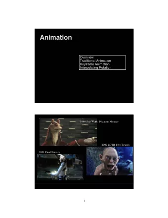
Keyframe animation Process of keyframing Keyframe interpolation Hermite and Bezier curves Splines Speed control Oldest keyframe animation Two conditions to make moving images in 19th century at
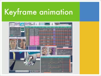
Keyframe animation
• Process of keyframing � • Keyframe interpolation � • Hermite and Bezier curves � • Splines � • Speed control
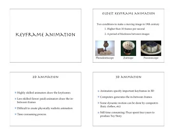
Oldest keyframe animation • Two conditions to make moving images in 19th century � • at least 10 frames per second � • a period of blackness between images
2D animation • Highly skilled animators draw the keyframes � • Less skilled (lower paid) animators draw the in-between frames � • Time consuming process � • Difficult to create physically realistic animation
3D animation • Animators specify important keyframes in 3D � • Computers generates the in-between frames � • Some dynamic motion can be done by computers (hair, clothes, etc) � • Still time consuming
General pipeline • Story board � • Keyframes � • Inbetweens � • Painting
Storyboards • The film in outline form � • specify the key scenes � • specify the camera moves and edits � • specify character gross motion � • Typically paper and pencil sketches on individual sheets taped on a wall
“A bug’s life”
The process of keyframing • Specify the keyframes � • Specify the type of interpolation � • linear, cubic, parametric curves � • Specify the speed profile of the interpolation � • constant velocity, ease-in-ease-out, etc � • Computer generates the in-between frames
A keyframe • In 2D animation, a keyframe is usually a single image � • In 3D animation, each keyframe is defined by a set of parameters
Keyframe parameters • What are the parameters? � • position and orientation � • body deformation � • facial features � • hair and clothing � • lights and cameras
• Process of keyframing � • Keyframe interpolation � • Hermite and Bezier curves � • Splines � • Speed control
In-between frames • Linear interpolation � • Cubic curve interpolation
Linear interpolation Linearly interpolate the parameters between keyframes t = 5 t = 10 t = 0 t = 15 end key start key x = x 0 + t − t 0 ( x 1 − x 0 ) t 1 − t 0 end time start time
Cubic curve interpolation We can use three cubic functions to represent a 3D curve Each function is defined with the range 0 ≤ t ≤ 1 bold: a vector or a matrix � Q ( t ) = [ x ( t ) y ( t ) z ( t )] italic: a scalar or vectors Q x ( t ) = a x t 3 + b x t 2 + c x t + d x a · b : inner product a × b : cross product Q y ( t ) = a y t 3 + b y t 2 + c y t + d y matrices Q z ( t ) = a z t 3 + b z t 2 + c z t + d z multiplication A · B : multiplication AB :
Compact representation Q ( t ) = [ Q x ( t ) Q y ( t ) Q z ( t )] Q x ( t ) = a x t 3 + b x t 2 + c x t + d x Q y ( t ) = a y t 3 + b y t 2 + c y t + d y Q z ( t ) = a z t 3 + b z t 2 + c z t + d z a x a y a z b x b y b z � t 3 t 2 � C = T = 1 t c x c y c z d x d y d z
Quiz Q ( t ) = [ Q x ( t ) Q y ( t ) Q z ( t )] a x a y a z b x b y b z Q x ( t ) = a x t 3 + b x t 2 + c x t + d x C = c x c y c z d x d y d z Q y ( t ) = a y t 3 + b y t 2 + c y t + d y Q z ( t ) = a z t 3 + b z t 2 + c z t + d z � t 3 t 2 � T = 1 t Which of the following is correct? 1. Q = C + T 2. Q = CT 3. Q = TC
Compact representation ⎡ ⎤ a x a y a z b x b y b z ⎢ ⎥ � t 3 t 2 � 1 Q ( t ) = ⎦ = TC t ⎢ ⎥ c x c y c z ⎣ d x d y d z d ˙ � � 3 t 2 2 t 1 0 dt Q ( t ) = C Q =
Determine coefficients How many constraints do we need to determine a cubic curve? 4 Two constraints come from end points, what about other two constraints? desired shape of the curve
Constraints on the cubics Redefine C as a product of the basis matrix M and the geometry matrix G C = M · G ⎡ ⎤ ⎡ ⎤ m 11 m 12 m 13 m 14 G 1 x G 1 y G 1 z � t 3 m 21 m 22 m 23 m 24 G 2 x G 2 y G 2 z 1 � ⎢ ⎥ ⎢ ⎥ t 2 Q ( t ) = t ⎢ ⎥ ⎢ ⎥ m 31 m 32 m 33 m 34 G 3 x G 3 y G 3 z ⎣ ⎦ ⎣ ⎦ m 41 m 42 m 43 m 44 G 4 x G 4 y G 4 z = T · M · G
• Process of keyframing � • Keyframe interpolation � • Hermite and Bezier curves � • Splines � • Speed control
Hermite curves • A Hermite curve is determined by � P 4 R 4 • endpoints P 1 and P 4 � • tangent vectors R 1 and R 4 at the P 1 R 1 endpoints � • Use these elements to construct geometry matrix P 1 x P 1 y P 1 z P 4 x P 4 y P 4 z G h = R 1 x R 1 y R 1 z R 4 x R 4 y R 4 z
Hermite basis matrix Given desired constraints: 1. endpoints meet P 1 and P 4 � � 0 0 0 1 Q (0) = · M h · G h = P 1 � � 1 1 1 1 Q (1) = · M h · G h = P 4 2. tangent vectors meet R 1 and R 4 ˙ � � 0 0 1 0 Q (0) = · M h · G h = R 1 ˙ � � 3 2 1 0 Q (1) = · M h · G h = R 4
Hermite basis matrix We can solve for basis matrix M h P 1 0 0 0 1 P 4 1 1 1 1 = G h = · M h · G h R 1 0 0 1 0 R 4 3 2 1 0 − 1 0 0 0 1 2 − 2 1 1 1 1 1 1 − 3 3 − 2 − 1 M h = = 0 0 1 0 0 0 1 0 3 2 1 0 1 0 0 0
Hermite Blending functions Let’s define B as a product of T and M ⎡ ⎤ 2 − 2 1 1 − 3 3 − 2 − 1 ⎢ ⎥ � t 3 t 2 � B h ( t ) = 1 t ⎢ ⎥ 0 0 1 0 ⎣ ⎦ 1 0 0 0 B h ( t ) indicates the weight of each element in G h B h ( t ) P 1 P 4 P 1 P 4 Q ( t ) = B h ( t ) · R 1 R 4 R 1 t R 4
Bézier curves Indirectly specify tangent vectors by specifying two intermediate points R 1 P 3 R 1 = 3( P 2 − P 1 ) P 4 P 2 R 4 = 3( P 4 − P 3 ) P 1 R 4 P 1 P 2 G b = P 3 P 4
Bézier basis matrix Establish the relation between Hermite and Bezier geometry vectors P 1 P 1 1 0 0 0 P 4 0 0 0 1 P 2 G h = = M hb · G b = R 1 − 3 3 0 0 P 3 R 4 P 4 0 0 − 3 3
Bézier basis matrix Q ( t ) = T · M h · G h = T · M h · ( M hb · G b ) = T · ( M h · M hb ) · G b = T · M b · G b − 1 3 − 3 1 3 − 6 3 0 M b = M h M hb = − 3 3 0 0 1 0 0 0 http://www.math.ucla.edu/~baker/java/hoefer/Bezier.htm
Bézier blending functions Bezier blending functions are also called Bernstein polynomials ⎡ ⎤ − 1 3 − 3 1 3 − 6 3 0 ⎢ ⎥ � t 3 t 2 � B b ( t ) = 1 t ⎢ ⎥ − 3 3 0 0 ⎣ ⎦ 1 0 0 0 B b ( t ) P 1 P 1 P 4 P 2 Q ( t ) = B b ( t ) · P 2 P 3 P 3 P 4 t
Complex curves What if we want to model a curve that passes through these points? Problem with higher order polynomials: Wiggly curves No local control
• Process of keyframing � • Keyframe interpolation � • Hermite and Bezier curves � • Splines � • Speed control
Splines • A piecewise polynomial that has locally very simple form, yet be globally flexible and smooth � • There are three nice properties of splines we’d like to have � • Continuity � • Local control � • Interpolation
Continuity • Cubic curves are continuous and differentiable � • We only need to worry about the derivatives at the endpoints when two curves meet
Continuity C 0 : points coincide, velocities don’t C 1 : points and velocities coincide What’s C 2 ? points, velocities and accelerations coincide
Local control • We’d like to have each control point on the spline only affect some well-defined neighborhood around that point � • Bezier and Hermite curves don’t have local control; moving a single control point affects the whole curve
Interpolation • We’d like to have a spline interpolating the control points so that the spline always passes through every control points � • Bezier curves do not necessarily pass through all the control points
B-splines • We can join multiple Bezier curves to create B- splines � • Ensure C 2 continuity when two curves meet
Continuity in B-splines Suppose we want to join two Bezier curves ( V 0 , V 1 , V 2 , V 3 ) and ( W 0 , W 1 , W 2 , W 3 ) so that C 2 continuity is met at the joint V 1 W 1 V 2 W 2 V 0 W 3 V 3 W 0 Q v (1) = Q w (0) V 3 = W 0 Q v (1) = ˙ ˙ Q w (0) V 3 − V 2 = W 1 − W 0 Q v (1) = ¨ ¨ Q w (0) V 1 − 2 V 2 + V 3 = W 0 − 2 W 1 + W 2 W 2 = V 1 + 4 V 3 − 4 V 2
Continuity in B-splines What does this derived equation mean geometrically? W 2 = V 1 + 4 V 3 − 4 V 2 What is the relationship between a, b and c, if a = 2b - c? W 0 = V 3 V 1 V 2 B 1 W 1 = 2 V 3 − V 2 V 3 = W 0 V 0 W 2 = V 1 + 4 V 3 − 4 V 2 W 1 = 2(2 V 3 − V 2 ) − (2 V 2 − V 1 ) W 2 = 2 W 1 − B 1 W 3 What is B 2 ? B 2
de Boor points Instead of specifying the Bezier control points, let’s specify the corners of the frames that form a B-spline These points are called de Boor points and the frames are called A-frames
Recommend
More recommend
Explore More Topics
Stay informed with curated content and fresh updates.
