Drawing Metro Maps using B ezier Curves Martin Fink Lehrstuhl f - PowerPoint PPT Presentation
Drawing Metro Maps using B ezier Curves Martin Fink Lehrstuhl f ur Informatik I Universit at W urzburg Joint work with Herman Haverkort, Martin N ollenburg, Maxwell Roberts, Julian Schuhmann & Alexander Wolff 1 /21 We
Drawing Metro Maps using B´ ezier Curves Martin Fink Lehrstuhl f¨ ur Informatik I Universit¨ at W¨ urzburg Joint work with Herman Haverkort, Martin N¨ ollenburg, Maxwell Roberts, Julian Schuhmann & Alexander Wolff 1 /21
We have . . . [N¨ ollenburg and Wolff, 2011] [Hong et al., 2006], [Stott et al., 2011] 2 /21
We want to create . . . [Roberts, 2007] 3 /21
Octilinear vs. Curvy Drawings metro line: polyline with bends (possibly in stations) very schematized 4 /21
Octilinear vs. Curvy Drawings metro line: polycurve without bends 4 /21
Octilinear vs. Curvy Drawings metro line: polycurve without bends [Roberts et al., 2012]: improved planning speed 4 /21
Octilinear vs. Curvy Drawings metro line: polycurve without bends [Roberts et al., 2012]: improved planning speed more artistic demand of Peter Eades! [GD’10] 4 /21
(Cubic) B´ ezier Curves parametric curves 5 /21
(Cubic) B´ ezier Curves parametric curves q ′ p ′ C p q R 2 C : [0, 1] → (1 − t ) 3 p + 3(1 − t ) 2 tp ′ + 3(1 − t ) t 2 q ′ + t 3 q t �→ 5 /21
(Cubic) B´ ezier Curves parametric curves leave vertices in direction of tangents q ′ p ′ C p q R 2 C : [0, 1] → (1 − t ) 3 p + 3(1 − t ) 2 tp ′ + 3(1 − t ) t 2 q ′ + t 3 q t �→ 5 /21
(Cubic) B´ ezier Curves parametric curves leave vertices in direction of tangents q ′ p ′ C p q R 2 curves share tangents C : [0, 1] → (1 − t ) 3 p + 3(1 − t ) 2 tp ′ + 3(1 − t ) t 2 q ′ + t 3 q fit smoothly together t �→ 5 /21
(Cubic) B´ ezier Curves parametric curves leave vertices in direction of tangents q ′ p ′ C p q R 2 curves share tangents C : [0, 1] → (1 − t ) 3 p + 3(1 − t ) 2 tp ′ + 3(1 − t ) t 2 q ′ + t 3 q fit smoothly together t �→ 5 /21
(Cubic) B´ ezier Curves parametric curves leave vertices in direction of tangents q ′ p ′ C p q R 2 curves share tangents C : [0, 1] → (1 − t ) 3 p + 3(1 − t ) 2 tp ′ + 3(1 − t ) t 2 q ′ + t 3 q fit smoothly together t �→ 5 /21
(Cubic) B´ ezier Curves parametric curves leave vertices in direction of tangents − → p C our representation: control point = q ′ � p ′ tangent + distance r C ( p ) C p q R 2 C : [0, 1] → (1 − t ) 3 p + 3(1 − t ) 2 tp ′ + 3(1 − t ) t 2 q ′ + t 3 q t �→ 5 /21
Previous Work [Brandes, Shubina, Tamassia, Wagner, 2001]: B´ ezier curves used for visualizing train connections. [Brandes, Shubina, Tamassia, 2000], [Brandes, Wagner, 1998] 6 /21
Previous Work [Brandes, Shubina, Tamassia, Wagner, 2001]: B´ ezier curves used for visualizing train connections. [Brandes, Shubina, Tamassia, 2000], [Brandes, Wagner, 1998] Our approach: – share tangents – move vertices 6 /21
Previous Work [Brandes, Shubina, Tamassia, Wagner, 2001]: B´ ezier curves used for visualizing train connections. [Brandes, Shubina, Tamassia, 2000], [Brandes, Wagner, 1998] Our approach: – share tangents – move vertices [Finkel and Tamassia, 2005]: Force-directed algorithm for drawing graphs with B´ ezier Curves 6 /21
Previous Work [Brandes, Shubina, Tamassia, Wagner, 2001]: B´ ezier curves used for visualizing train connections. [Brandes, Shubina, Tamassia, 2000], [Brandes, Wagner, 1998] Our approach: – share tangents – move vertices [Finkel and Tamassia, 2005]: Force-directed algorithm for drawing graphs with B´ ezier Curves Method: Control-points as extra vertices. 6 /21
Previous Work [Brandes, Shubina, Tamassia, Wagner, 2001]: B´ ezier curves used for visualizing train connections. [Brandes, Shubina, Tamassia, 2000], [Brandes, Wagner, 1998] Our approach: – share tangents – move vertices [Finkel and Tamassia, 2005]: Force-directed algorithm for drawing graphs with B´ ezier Curves Method: Control-points as extra vertices. our approach: control points are no vertices 6 /21
Our Approach use B´ ezier curves for representing edges 7 /21
Our Approach use B´ ezier curves for representing edges use force-directed approach 7 /21
Obtaining an Initial Drawing with Curves geographic input 8 /21
Obtaining an Initial Drawing with Curves straight-line drawing 8 /21
Obtaining an Initial Drawing with Curves straight-line drawing alternative: use octilinear drawing 8 /21
Obtaining an Initial Drawing with Curves approximation by B´ ezier Curves 8 /21
Obtaining an Initial Drawing with Curves approximation by B´ ezier Curves put control points close to vertex use common tangents 8 /21
Structure of the Algorithm while the drawing changes compute forces on vertices compute forces on curves apply forces simplify the drawing perform post-processing simplification 9 /21
Structure of the Algorithm while the drawing changes compute forces on vertices stop if displacement is small compute forces on curves apply forces simplify the drawing perform post-processing simplification 9 /21
Structure of the Algorithm while the drawing changes compute forces on vertices compute forces on curves apply forces simplify the drawing perform post-processing simplification 9 /21
Structure of the Algorithm while the drawing changes compute forces on vertices compute forces on curves sum up to desired changes apply forces simplify the drawing perform post-processing simplification 9 /21
Structure of the Algorithm while the drawing changes compute forces on vertices compute forces on curves apply forces simplify the drawing avoid intersections perform post-processing simplification ✗ 9 /21
Structure of the Algorithm while the drawing changes compute forces on vertices compute forces on curves apply forces simplify the drawing perform post-processing simplification merge curves around deg-2 vertex 9 /21
Structure of the Algorithm while the drawing changes compute forces on vertices compute forces on curves apply forces simplify the drawing perform post-processing simplification merge 4 curves to 2 9 /21
Forces – Vertices – repulsion 10 /21
Forces – Vertices – repulsion – attraction of adjacent vertices 10 /21
Forces – Vertices – repulsion – attraction of adjacent vertices reuse forces from Fruchterman-Rheingold 10 /21
Forces – Vertices – repulsion – attraction of adjacent vertices desired edge length = const · (# intermediate stops + 1) 10 /21
Forces – Vertices – repulsion – attraction of adjacent vertices – attraction to geographic position 10 /21
Forces – Shape of Curves ✗ 11 /21
Forces – Shape of Curves ✗ ✗ 11 /21
Forces – Shape of Curves ✗ � ✗ 11 /21
Forces – Shape of Curves ✗ � ✗ 11 /21
Forces – Shape of Curves a b ✗ � ✗ b ≈ 1 a distances: 3 use Fruchterman-Rheingold-like spring force 11 /21
Forces – Straightening Curves ✗ 12 /21
Forces – Straightening Curves ✗ � 12 /21
Forces – Straightening Curves ✗ � straight-line segment = simplest curve 12 /21
Forces – Straightening Curves ✗ � straight-line segment = simplest curve t move vertex v towards tangent v t u v 12 /21
Forces – Straightening Curves ✗ � straight-line segment = simplest curve t move vertex v towards tangent v t v t rotate tangent towards straight-line α u v 12 /21
Forces – Straightening Curves adding up rotational forces ✗ � straight-line segment = simplest curve t move vertex v towards tangent v t v t rotate tangent towards straight-line α u v 12 /21
Forces – Straightening Curves adding up rotational forces ✗ � straight-line segment = simplest curve t move vertex v towards tangent v t v t rotate tangent towards straight-line law of the lever : α force weighted by distance u v 12 /21
Forces – Angular Resolution ✗ 13 /21
Forces – Angular Resolution ✗ � 13 /21
Forces – Angular Resolution α ✗ � tangents repelling each other force = const. · 1 α 13 /21
Avoiding Intersections ✗ 14 /21
Avoiding Intersections ✗ � 14 /21
Merging Curves intermediate stop 15 /21
Merging Curves intermediate stop keep control points 15 /21
Merging Curves intermediate stop keep control points different distances for keeping the drawing crossing-free 15 /21
Merging Curves intermediate stop keep control points different distances for keeping the drawing crossing-free Tests: not necessary 15 /21
Merging Curves in Interchange Stations merge 4 curves to 2 16 /21
Merging Curves in Interchange Stations merge 4 curves to 2 station = crossing 16 /21
Merging Curves in Interchange Stations merge 4 curves to 2 edge proportions should be kept approximately testing different control point distances necessary 16 /21
Recommend
More recommend
Explore More Topics
Stay informed with curated content and fresh updates.
