KernGPLM A Package for Kernel-Based Fitting of Aim of this Talk - PowerPoint PPT Presentation

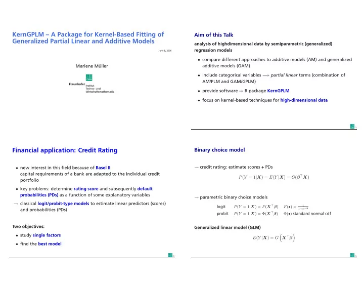
KernGPLM – A Package for Kernel-Based Fitting of Aim of this Talk Generalized Partial Linear and Additive Models analysis of highdimensional data by semiparametric (generalized) regression models June 8, 2006 • compare different approaches to additive models (AM) and generalized additive models (GAM) Marlene Müller • include categorical variables = ⇒ partial linear terms (combination of AM/PLM and GAM/GPLM) • provide software ⇒ R package KernGPLM • focus on kernel-based techniques for high-dimensional data 1 Financial application: Credit Rating Binary choice model → credit rating: estimate scores + PDs • new interest in this field because of Basel II : capital requirements of a bank are adapted to the individual credit P ( Y = 1 | X ) = E ( Y | X ) = G ( β ⊤ X ) portfolio • key problems: determine rating score and subsequently default probabilities (PDs) as a function of some explanatory variables → parametric binary choice models → classical logit/probit-type models to estimate linear predictors (scores) P ( Y = 1 | X ) = F ( X ⊤ β ) 1 logit F ( • ) = and probabilities (PDs) 1+ e −• P ( Y = 1 | X ) = Φ( X ⊤ β ) probit Φ( • ) standard normal cdf Two objectives: Generalized linear model (GLM) • study single factors � � X ⊤ β E ( Y | X ) = G • find the best model 2 3

Data Example: Credit Data Data Example: Logit (with interaction) References: Fahrmeir/Hamerle (1984); Fahrmeir & Tutz (1995) • default indicator: Y ∈ { 0 , 1 } , where 1 = default • explanatory variables: 15000 personal characteristics, credit history, credit characteristics S o re p revious − 0 . 310 · emplo y ed + 0 . 566 ⋆⋆ · (d9-12) • sample size: 1000 (stratified sample with 300 defaults) AMOUNT 10000 (d12-18) + 0 . 981 ⋆⋆⋆ · (d18-24) + 1 . 550 ⋆⋆⋆ · (d > 24) m Estimated (Logit) Scores savings − 0 . 363 ⋆⋆ · purp ose + 0 . 660 ⋆⋆⋆ · house AMOUNT 5000 amount − 0 . 0942 ⋆⋆ · age + 0 . 0000000173 ⋆⋆ · amount 2 1 . 334 − 0 . 763 ⋆⋆⋆ · = AGE age 2 + 0 . 00000236 · (amount · age) +0 . 898 ⋆⋆ · 0 − 0 . 984 ⋆⋆⋆ · 20 30 40 50 60 70 − 0 . 000251 ⋆⋆ · AGE credit default on AGE and AMOUNT using quadratic and interaction terms, left: +0 . 000833 ⋆ · surface and right: contours of the fitted score function ⋆ , ⋆⋆ , ⋆⋆⋆ denote significant coefficients at the 10%, 5%, 1% level, respectively 4 5 Semiparametric Models Data Example: GPLM • local regression E ( Y | T ) = G { m ( T ) } , m nonparametric 15000 • generalized partial linear model (GPLM) AMOUNT 10000 m � � X ⊤ β + m ( T ) E ( Y | X , T ) = G m nonparametric AMOUNT 5000 • generalized additive partial linear model (semiparametric GAM) AGE 0   p 20 30 40 50 60 70   �  β 0 + X ⊤ β + E ( Y | X , T ) = G m j ( T j ) m j nonparametric AGE  j =1 credit default on AGE and AMOUNT using a nonparametric function, left: surface and right: contours of the fitted score function on AGE and AMOUNT Some references: Loader (1999), Hastie and Tibshirani (1990), Härdle et al. (2004), Green and Silverman (1994) 6 7

Estimation Approaches for GPLM/GAM Estimation of the GPLM : generalized Speckman estimator • partial linear model (identity G ) E ( Y | X , T ) = X T β + m ( T ) • GPLM: ⋆ generalization of Speckman’s estimator (type of profile likelihood) m new = ⇒ = S ( Y − X β ) ⋆ backfitting for two additive components and local scoring X T e X ) − 1 e X T e β new ( e = Y References: (PLM) Speckman (1988), Robinson (1988); (PLM/splines) Schimek (2000), Eubank et al. (1998), • generalized partial linear model Schimek (2002); (GPLM) Severini and Staniswalis (1994), Müller (2001) E ( Y | X , T ) = G { X T β + m ( T ) } • semiparametric GAM: ⋆ [ modified | smooth ] backfitting and local scoring = ⇒ above for adjusted dependent variable ⋆ marginal [ internalized ] integration Z = X β + m − W − 1 v , References: v = ( ℓ ′ i ) , W = diag( ℓ ′′ (marginal integraton) Tjøstheim and Auestad (1994), Chen et al. (1996), i ) Hengartner et al. (1999), Hengartner and Sperlich (2005); (backfitting) Buja et al. (1989), Mammen et al. (1999), Nielsen and Sperlich (2005) References: Severini and Staniswalis (1994) 8 9 Estimation of the GAM Comparison of Algorithms   p   �  β 0 + X ⊤ β + E ( Y | X , T ) = G m j ( T j ) m j nonparametric parametric step nonparametric step est. matrix  j =1 β new = ( e X T W e X ) − 1 e X T W e m new = S ( Z − X β ) η = R S Z Speckman Z • classical backfitting: fit single components by regression on the residuals w.r.t. β new = ( X T W e X ) − 1 X T W e m new = S ( Z − X β ) η = R B Z Backfitting Z the other components β new = ( X T W e X ) − 1 X T W e m new = ... η = R P Z Profile Z • modified backfitting: first project on the linear space spanned by all regressors and then nonparametrically fit the partial residuals Speckman/Backfitting: X = ( I − S ) X , e e Z = ( I − S ) Z , S weighted smoother matrix • marginal (internalized) integration: estimate the marginal effect by integrating a full dimensional nonparametric regression estimate Profile Likelihood: ⇒ original proposal is computationally intractable: O ( n 3 ) X = ( I − S P ) X , e Z = ( I − S P ) Z , S P weighted (different) smoother matrix = e = ⇒ choice of nonparametric estimate is essential: marginal internalized References: Severini and Staniswalis (1994), Müller (2001) integration 10 11

Simulation Example: True Additive Function Simulation Example: True Non-Additive Function Backfit / Component 1 Backfit / Component 2 Backfit / Component 1 Backfit / Component 2 0.5 0.5 • B – classical • B – classical 0.0 0.0 0.0 0.0 −0.5 • B – modified • B – modified −0.5 −0.5 −1.0 −0.5 m[o, j] m[o, j] m[o, j] m[o, j] −1.5 −1.0 −1.0 −2.0 −1.0 −1.5 −2.5 −1.5 −1.5 −3.0 −2.0 −2 0 2 4 −2 0 2 4 6 8 10 12 −2 0 2 4 −3 −2 −1 0 1 2 3 4 t[o, j] t[o, j] t[o, j] t[o, j] Margint / Component 1 Margint / Component 2 Margint / Component 1 Margint / Component 2 0.5 0.5 0.0 0.0 0.0 • M – classical 0.0 • M – classical −0.5 −0.5 −0.5 −1.0 • M – pdf estimate 1 • M – pdf estimate 1 −0.5 m[o, j] m[o, j] m[o, j] m[o, j] −1.5 −1.0 • M – pdf estimate 2 • M – pdf estimate 2 −1.0 −2.0 −1.0 −1.5 −2.5 • M – normal pdfs • M – normal pdfs −1.5 −1.5 −3.0 −2.0 −2 0 2 4 −2 0 2 4 6 8 10 12 −2 0 2 4 −3 −2 −1 0 1 2 3 4 t[o, j] t[o, j] t[o, j] t[o, j] Marginal integration – as initialization for backfitting Marginal integration – estimate of marginal effects 12 13 Summary Comparison of Algorithms • consistency of marginal integration: • GPLM and semiparametric GAM are natural extensions of the GLM ⇒ if underlying function is truly additive, backfitting outperforms • large amount of data is needed for estimating marginal effects marginal integration ⇒ R package KernGPLM with routines for ⇒ consider marginal integration to initialize backfitting (replacing the usual zero-functions ⋆ (kernel based) generalized partial linear and additive models ⋆ additive components by [ modified ] backfitting + local scoring • comparison of backfitting and marginal integration: ⋆ additive components by marginal [ internalized ] integration ⇒ marginal integration indeed estimates marginal effects, but large number of observations is needed • possible extensions: ⇒ estimation method of the instruments is essential, dimension ⋆ smooth backfitting reduction techniques are required ⋆ externalized marginal integration 14 15