Kernel Methods CE-717: Machine Learning Sharif University of - PowerPoint PPT Presentation
Kernel Methods CE-717: Machine Learning Sharif University of Technology Fall 2019 Soleymani Not linearly separable data } Noisy data or overlapping classes 2 } (we discussed about it: soft margin) } Near linearly separable 1 }
Kernel Methods CE-717: Machine Learning Sharif University of Technology Fall 2019 Soleymani
Not linearly separable data } Noisy data or overlapping classes 𝑦 2 } (we discussed about it: soft margin) } Near linearly separable 𝑦 1 } Non-linear decision surface 𝑦 2 } Transform to a new feature space 2 𝑦 1
Nonlinear SVM } Assume a transformation 𝜚: ℝ ' → ℝ ) on the feature space 𝝔 𝒚 = [𝜚 , (𝒚), . . . , 𝜚 ) (𝒚)] } 𝒚 → 𝝔 𝒚 {𝜚 , (𝒚),...,𝜚 ) (𝒚)} : set of basis functions (or features) 𝜚 < 𝒚 : ℝ ' → ℝ } Find a hyper-plane in the transformed feature space: 𝜚 / (𝒚) 𝑦 2 𝜚: 𝒚 → 𝝔 𝒚 𝒙 2 𝝔 𝒚 + 𝑥 5 = 0 𝑦 1 𝜚 , (𝒚) 3
Soft-margin SVM in a transformed space: Primal problem } Primal problem: H 1 2 𝒙 / + 𝐷 E 𝜊 G min 𝒙,B C GI, 𝒙 2 𝝔(𝒚 G ) + 𝑥 5 ≥ 1 − 𝜊 G 𝑜 = 1, … , 𝑂 s. t. 𝑧 G 𝜊 G ≥ 0 } 𝒙 ∈ ℝ ) : the weights that must be found } If 𝑛 ≫ 𝑒 (very high dimensional feature space) then there are many more parameters to learn 4
Soft-margin SVM in a transformed space: Dual problem } Optimization problem: H H H − 1 2 E E 𝛽 G 𝛽 ) 𝑧 (G) 𝑧 ()) 𝝔 𝒚 (G) 2 𝝔 𝒚 ()) max E 𝛽 G 𝜷 GI, GI, )I, 𝛽 G 𝑧 (G) = 0 H ∑ Subject to } GI, 0 ≤ 𝛽 G ≤ 𝐷 𝑜 = 1, … , 𝑂 } } If we have inner products 𝝔 𝒚 (<) 2 𝝔 𝒚 (\) , only 𝜷 = [𝛽 , , … , 𝛽 H ] needs to be learnt. } not necessary to learn 𝑛 parameters as opposed to the primal problem 5
� Classifying a new data ] = 𝑡𝑗𝑜 𝑥 5 + 𝒙 2 𝝔(𝒚) 𝑧 𝛽 G 𝑧 (G) 𝝔(𝒚 (G) ) where 𝒙 = ∑ b c d5 and 𝑥 5 = 𝑧 (e) − 𝒙 2 𝝔(𝒚 (e) ) 6
Kernel SVM } Learns linear decision boundary in a high dimension space without explicitly working on the mapped data } Let 𝝔 𝒚 2 𝝔 𝒚 f = 𝐿(𝒚, 𝒚 f ) (kernel) } Example: 𝒚 = 𝑦 , , 𝑦 / and second-order 𝝔 : / , 𝑦 / / , 𝑦 , 𝑦 / 𝝔 𝒚 = 1, 𝑦 , , 𝑦 / , 𝑦 , 𝐿 𝒚, 𝒚 f f + 𝑦 / 𝑦 / f + 𝑦 , f/ + 𝑦 / f/ + 𝑦 , 𝑦 , / 𝑦 , / 𝑦 / f 𝑦 / 𝑦 / f = 1 + 𝑦 , 𝑦 , 7
� � � � � � Kernel trick } Compute 𝐿 𝒚, 𝒚 f without transforming 𝒚 and 𝒚′ } Example: Consider 𝐿 𝒚, 𝒚 f = 1 + 𝒚 2 𝒚 f / f + 𝑦 / 𝑦 / f / = 1 + 𝑦 , 𝑦 , f + 2𝑦 / 𝑦 / f + 𝑦 , f/ + 𝑦 / f/ + 2𝑦 , 𝑦 , / 𝑦 , / 𝑦 / f 𝑦 / 𝑦 / f = 1 + 2𝑦 , 𝑦 , This is an inner product in: / , 𝑦 / / , 𝝔 𝒚 = 1, 2 𝑦 , , 2 𝑦 / , 𝑦 , 2 𝑦 , 𝑦 / f , f , 𝑦′ , / , 𝑦′ / / , f 𝑦 / f 𝝔 𝒚′ = 1, 2 𝑦 , 2 𝑦 / 2 𝑦 , 8
� � � � � � Polynomial kernel: Degree two } We instead use 𝐿(𝒚, 𝒚′) = 𝒚 2 𝒚′ + 1 / that corresponds to: 𝑒 -dimensional feature space 𝒚 = 𝑦 , , … ,𝑦 ' 2 𝝔 𝒚 2 / , . . , 𝑦 ' / , = 1, 2 𝑦 , , … , 2 𝑦 ' , 𝑦 , 2 𝑦 , 𝑦 / , … , 2 𝑦 , 𝑦 ' , 2 𝑦 / 𝑦 i , … , 2 𝑦 'j, 𝑦 ' 9
� � � Polynomial kernel } This can similarly be generalized to d-dimensioan 𝒚 and 𝜚 s are polynomials of order 𝑁 : 𝐿 𝒚, 𝒚 f = 1 + 𝒚 2 𝒚 f l f + 𝑦 / 𝑦 / f + ⋯ + 𝑦 ' 𝑦 ' f l = 1 + 𝑦 , 𝑦 , } Example: SVM boundary for a polynomial kernel } 𝑥 5 + 𝒙 2 𝝔 𝒚 = 0 2 𝝔 𝒚 = 0 𝛽 < 𝑧 (<) 𝝔 𝒚 < } ⇒ 𝑥 5 + ∑ b o d5 𝛽 < 𝑧 (<) 𝑙(𝒚 < , 𝒚) = 0 } ⇒ 𝑥 5 + ∑ b o d5 l Boundary is a 𝛽 < 𝑧 (<) 1 + 𝒚 (<) q 𝒚 } ⇒ 𝑥 5 + ∑ = 0 b o d5 polynomial of order 𝑁 10
Why kernel? } kernel functions 𝐿 can indeed be efficiently computed, with a cost proportional to 𝑒 (the dimensionality of the input) instead of 𝑛 . } Example: consider the second-order polynomial transform: / , 𝑦 , 𝑦 / , … , 𝑦 ' 𝑦 ' 2 𝝔 𝒚 = 1, 𝑦 , , … , 𝑦 ' , 𝑦 , 𝑟 = 1 + 𝑒 + 𝑒 / ' ' ' f f 𝑦 \ f 𝝔 𝒚 2 𝝔 𝒚′ = 1 + E 𝑦 < 𝑦 < + E E 𝑦 < 𝑦 \ 𝑦 < 𝑃(𝑟) \I, <I, <I, ' ' f f E 𝑦 < 𝑦 < × E 𝑦 \ 𝑦 \ <I, \I, 𝝔 𝒚 2 𝝔 𝒚′ = 1 + 𝑦 2 𝑦 f + 𝑦 2 𝑦 f / 𝑃(𝑒) 11
Gaussian or RBF kernel } If 𝐿 𝒚, 𝒚 f is an inner product in some transformed space of x, it is good 𝒚j𝒚 w x } 𝐿 𝒚, 𝒚 f = exp (− ) y } Take one dimensional case with 𝛿 = 1 : 𝐿 𝑦, 𝑦 f = exp − 𝑦 − 𝑦 f / = exp −𝑦 / exp −𝑦′ / exp 2𝑦𝑦′ } = exp −𝑦 / exp −𝑦′ / E 2 { 𝑦 { 𝑦′ { 𝑙! {I5 12
Some common kernel functions } Linear: 𝑙(𝒚, 𝒚 f ) = 𝒚 2 𝒚′ } Polynomial: 𝑙 𝒚, 𝒚 f = (𝒚 2 𝒚 f + 1) l 𝒚j𝒚 w x } Gaussian: 𝑙 𝒚, 𝒚 f = exp (− ) y } Sigmoid: 𝑙 𝒚, 𝒚 f = tanh (𝑏𝒚 2 𝒚 f + 𝑐) 13
Kernel formulation of SVM } Optimization problem: H H H − 1 2 E E 𝛽 G 𝛽 ) 𝑧 (G) 𝑧 ()) 𝝔 𝒚 (G) 2 𝝔 𝒚 ()) 𝑙(𝒚 G , 𝒚 ()) ) max E 𝛽 G 𝜷 GI, GI, )I, 𝛽 G 𝑧 (G) = 0 H ∑ Subject to } GI, 0 ≤ 𝛽 G ≤ 𝐷 𝑜 = 1, … , 𝑂 } 𝑧 , 𝑧 , 𝐿 𝒚 , , 𝒚 , 𝑧 , 𝑧 H 𝐿 𝒚 H , 𝒚 , ⋯ 𝑹 = ⋮ ⋱ ⋮ 𝑧 H 𝑧 , 𝐿 𝒚 H , 𝒚 , 𝑧 H 𝑧 H 𝐿 𝒚 H , 𝒚 H ⋯ 14
� � � Classifying a new data ] = 𝑡𝑗𝑜 𝑥 5 + 𝒙 2 𝝔(𝒚) 𝑧 𝛽 G 𝑧 (G) 𝝔(𝒚 (G) ) where 𝒙 = ∑ b c d5 and 𝑥 5 = 𝑧 (e) − 𝒙 2 𝝔(𝒚 (e) ) 𝑙(𝒚 G , 𝒚) 2 ] = 𝑡𝑗𝑜 𝑥 5 + E 𝛽 G 𝑧 G 𝝔 𝒚 G 𝑧 𝝔(𝒚) b c d5 𝑙(𝒚 G , 𝒚 (e) ) 2 𝑥 5 = 𝑧 (e) − E 𝛽 G 𝑧 G 𝝔 𝒚 G 𝝔 𝒚 e b c d5 15
� Gaussian kernel } Example: SVM boundary for a Gaussian kernel } Considers a Gaussian function around each data point. 𝒚j𝒚 (o) x 𝛽 < 𝑧 (<) exp } 𝑥 5 + ∑ (− ) = 0 b o d5 „ } SVM + Gaussian Kernel can classify any arbitrary training set } Training error is zero when 𝜏 → 0 ¨ All samples become support vectors (likely overfiting) 16
Hard margin Example } For narrow Gaussian (large 𝜏 ), even the protection of a large margin cannot suppress overfitting. Y. Abu-Mostafa et. Al, 2012 17
� SVM Gaussian kernel: Example (− 𝒚 − 𝒚 (<) / 𝛽 < 𝑧 (<) exp 𝑔 𝒚 = 𝑥 5 + E ) 2𝜏 / b o d5 18 This example has been adopted from Zisserman’s slides
SVM Gaussian kernel: Example 19 This example has been adopted from Zisserman’s slides
SVM Gaussian kernel: Example 20 This example has been adopted from Zisserman’s slides
SVM Gaussian kernel: Example 21 This example has been adopted from Zisserman’s slides
SVM Gaussian kernel: Example 22 This example has been adopted from Zisserman’s slides
SVM Gaussian kernel: Example 23 This example has been adopted from Zisserman’s slides
SVM Gaussian kernel: Example 24 This example has been adopted from Zisserman’s slides
Kernel trick: Idea } Kernel trick → Extension of many well-known algorithms to kernel-based ones } By substituting the dot product with the kernel function } 𝑙 𝒚, 𝒚 f = 𝝔 𝒚 2 𝝔(𝒚′) } 𝑙 𝒚, 𝒚 f shows the dot product of 𝒚 and 𝒚 f in the transformed space. } Idea: when the input vectors appears only in the form of dot products, we can use kernel trick } Solving the problem without explicitly mapping the data } Explicit mapping is expensive if 𝝔 𝒚 is very high dimensional 25
Kernel trick: Idea (Cont’d) } Instead of using a mapping 𝝔: 𝒴 ← ℱ to represent 𝒚 ∈ 𝒴 by 𝝔(𝒚) ∈ ℱ , a kernel function 𝑙: 𝒴×𝒴 → ℝ is used. } We specify only an inner product function between points in the transformed space (not their coordinates) } In many cases, the inner product in the embedding space can be computed efficiently. 26
� Constructing kernels } Construct kernel functions directly } Ensure that it is a valid kernel } Corresponds to an inner product in some feature space. } Example: 𝑙(𝒚, 𝒚 f ) = 𝒚 2 𝒚 f / / 2 for 𝒚 = / , } Corresponding mapping: 𝝔 𝒚 = 𝑦 , 2 𝑦 , 𝑦 / , 𝑦 / 𝑦 , , 𝑦 / 2 } We need a way to test whether a kernel is valid without having to construct 𝝔 𝒚 27
Construct Valid Kernels 𝑑 > 0 , 𝑙 1 : valid kernel • 𝑔(. ) : any function • 𝑟(. ) : a polynomial with coefficients ≥ 0 • 𝑙 1 , 𝑙 2 : valid kernels • 𝝔(𝒚) : a function from 𝒚 to ℝ l • 𝑙3(. , . ) : a valid kernel in ℝ l 𝑩 : a symmetric positive semi-definite • matrix 𝒚 Ž and 𝒚 • are variables (not necessarily • disjoint) with 𝒚 = (𝒚 Ž , 𝒚 • ) , and 𝑙 Ž and 𝑙 • are valid kernel functions over their respective spaces. [Bishop] 28
Recommend
More recommend
Explore More Topics
Stay informed with curated content and fresh updates.
