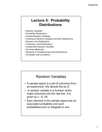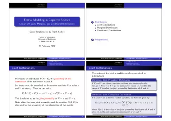
Joint Probability Distributions In many random experiments, more - PowerPoint PPT Presentation

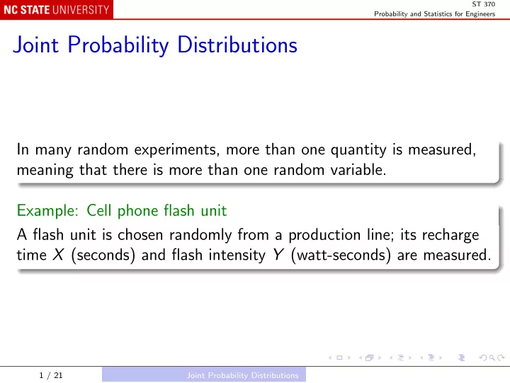
ST 370 Probability and Statistics for Engineers Joint Probability Distributions In many random experiments, more than one quantity is measured, meaning that there is more than one random variable. Example: Cell phone flash unit A flash unit is chosen randomly from a production line; its recharge time X (seconds) and flash intensity Y (watt-seconds) are measured. 1 / 21 Joint Probability Distributions

ST 370 Probability and Statistics for Engineers Example: Bernoulli trials X 1 is the indicator of success on the first trial: � 1 success on first trial X 1 = 0 otherwise and X 2 , X 3 , . . . , the indicators for the other trials, are all random variables. 2 / 21 Joint Probability Distributions

ST 370 Probability and Statistics for Engineers Two or More Random Variables To make probability statements about several random variables, we need their joint probability distribution. Discrete random variables If X and Y are discrete random variables, they have a joint probability mass function f XY ( x i , y j ) = P ( X = x i and Y = y j ) . 3 / 21 Joint Probability Distributions Two or More Random Variables

ST 370 Probability and Statistics for Engineers Example: Mobile response time A mobile web site is accessed from a smart phone; X is the signal strength, in number of bars, and Y is response time, to the nearest second. x = Number of bars 1 2 3 y = Response time 4+ 0.15 0.10 0.05 3 0.02 0.10 0.05 2 0.02 0.03 0.20 1 0.01 0.02 0.25 4 / 21 Joint Probability Distributions Two or More Random Variables

ST 370 Probability and Statistics for Engineers Continuous random variables If X and Y are continuous random variables, they have a joint probability density function f XY ( x , y ), with the interpretation � b � d P ( a ≤ X ≤ b and c ≤ Y ≤ d ) = f XY ( x , y ) dy dx . a c If one random variable is discrete and the other is continuous, the joint distribution is more complex. In all cases, they have a joint cumulative distribution function F XY ( x , y ) = P ( X ≤ x and Y ≤ y ) . 5 / 21 Joint Probability Distributions Two or More Random Variables

ST 370 Probability and Statistics for Engineers Marginal probability distributions Since X is a random variable, it also has its own probability distribution, ignoring the value of Y , called its marginal probability distribution. Discrete case: f X ( x i ) = P ( X = x i ) = P ( X = x i and Y takes any value) � = P ( X = x i , Y = y j ) j � = f XY ( x i , y j ) , and similarly j � f Y ( y j ) = f XY ( x i , y j ) . i 6 / 21 Joint Probability Distributions Two or More Random Variables

ST 370 Probability and Statistics for Engineers Example: Mobile response time Marginal distributions of X and Y : x = Number of bars 1 2 3 Marginal y = Response time 4+ 0.15 0.10 0.05 0.30 3 0.02 0.10 0.05 0.17 2 0.02 0.03 0.20 0.25 1 0.01 0.02 0.25 0.28 Marginal 0.20 0.25 0.55 7 / 21 Joint Probability Distributions Two or More Random Variables

ST 370 Probability and Statistics for Engineers Continuous case: � ∞ f X ( x ) = f XY ( x , y ) dy . −∞ and � ∞ f Y ( y ) = f XY ( x , y ) dx . −∞ 8 / 21 Joint Probability Distributions Two or More Random Variables

ST 370 Probability and Statistics for Engineers Cumulative distribution: F X ( x ) = P ( X ≤ x ) = P ( X ≤ x , Y takes any value) = P ( X ≤ x , Y < ∞ ) = F XY ( x , ∞ ) and F Y ( y ) = F XY ( ∞ , y ) . 9 / 21 Joint Probability Distributions Two or More Random Variables

ST 370 Probability and Statistics for Engineers Conditional probability distributions Suppose that X and Y are discrete random variables, and that we observe the value of X : X = x i for one of its values x i . What does that tell us about Y ? Recall conditional probability: P ( Y = y j | X = x i ) = P ( Y = y j ∩ X = x i ) P ( X = x i ) = f XY ( x i , y j ) . f X ( x i ) This is the conditional probability mass function of Y given X = x i , written f Y | X ( y | x i ). 10 / 21 Joint Probability Distributions Two or More Random Variables

ST 370 Probability and Statistics for Engineers Example: Mobile response time Conditional distributions of Y given X : x = Number of bars 1 2 3 y = Response time 4+ 0.750 0.400 0.091 3 0.100 0.400 0.091 2 0.100 0.120 0.364 1 0.050 0.080 0.454 Total 1 1 1 11 / 21 Joint Probability Distributions Two or More Random Variables

ST 370 Probability and Statistics for Engineers When X and Y are continuous random variables, the conditional probability density function of Y given X is also defined as a ratio: f Y | X ( y | x ) = f XY ( x , y ) , f X ( x ) but the reason is less clear: P ( X = x ) = 0, so we cannot simply divide the joint probability by the marginal probability. One approach is to condition on X being near to x , say x − δ x ≤ X ≤ x + δ x for some small δ x > 0, and take the limit as δ x ↓ 0. 12 / 21 Joint Probability Distributions Two or More Random Variables

ST 370 Probability and Statistics for Engineers Independent random variables In some situations, knowing the value of X gives no information about the value of Y . So the conditional distribution of Y given X is the same as the marginal distribution of Y : f Y | X ( y | x ) = f Y ( y ) . In this case, X and Y are said to be independent random variables. 13 / 21 Joint Probability Distributions Two or More Random Variables

ST 370 Probability and Statistics for Engineers But f Y | X ( y | x ) = f XY ( x , y ) , f X ( x ) so when X and Y are independent f XY ( x , y ) = f Y ( y ) , f X ( x ) or f XY ( x , y ) = f X ( x ) f Y ( y ) . This is true for either the probability density function or the probability mass function. 14 / 21 Joint Probability Distributions Two or More Random Variables

ST 370 Probability and Statistics for Engineers So for independent random variables, it is enough to know the marginal probability distributions: the joint probability distribution is just the product of the marginal functions. Example: Cell phone flash unit The recharge time X and flash intensity Y may not be independent: they are both affected by the quality of components such as capacitors, and a defective component may cause both a long recharge time and a low flash intensity. Example: Bernoulli trials We assume that the trials are independent, so the indicator variables X 1 , X 2 , . . . are also independent. 15 / 21 Joint Probability Distributions Two or More Random Variables

ST 370 Probability and Statistics for Engineers Designed experiments When you carry out a designed experiment, such as the replicated two-factor case Y i , j , k = µ + τ i + β j + ( τβ ) i , j + ǫ i , j , k , good technique will ensure that the result of any one run is unaffected by results of other runs. You would then assume that the responses Y i , j , k , i = 1 , . . . , a , j = 1 , . . . , b , k = 1 , . . . , n are independent random variables. 16 / 21 Joint Probability Distributions Two or More Random Variables

ST 370 Probability and Statistics for Engineers Equivalently, you could assume that the random noise terms ǫ i , j , k , i = 1 , . . . , a , j = 1 , . . . , b , k = 1 , . . . , n are independent. We always assume that the noise terms have zero expected value: E ( ǫ i , j , k ) = 0 , and usually also a common variance: V ( ǫ i , j , k ) = σ 2 . 17 / 21 Joint Probability Distributions Two or More Random Variables

ST 370 Probability and Statistics for Engineers In order to find the probability distributions of statistics like the t -ratio and the F -ratio, we shall also assume that the noise terms have Gaussian distributions; that is, ǫ i , j , k , i = 1 , . . . , a , j = 1 , . . . , b , k = 1 , . . . , n are independent random variables, each distributed as N (0 , σ 2 ). The joint distribution of these a × b × n random variables is determined by their common N (0 , σ 2 ) marginal distribution and the assumption of independence. 18 / 21 Joint Probability Distributions Two or More Random Variables

ST 370 Probability and Statistics for Engineers Residual Plots The probability distributions of statistics like the t -ratio and the F -ratio are derived under these assumptions about the random noise terms ǫ , so we should try to verify that the assumptions actually hold. We observe the responses Y , but the parameters µ and so on are unknown, so we cannot compute the noise terms ǫ . The best we can do is replace the parameters by their estimates, and compute the residuals β j + � τ i + ˆ e i , j , k = y i , j , k − (ˆ µ + ˆ ( τβ ) i , j ) = y i , j , k − ˆ y i , j , k . 19 / 21 Joint Probability Distributions Residual Plots

ST 370 Probability and Statistics for Engineers Four plots of the residuals are often used to look for departures from the assumptions: Residuals vs Fitted values: If E ( ǫ ) = 0, the residuals should vary around 0, with no pattern; curvature would suggest that second-order terms are needed. Normal quantile-quantile plot: If the noise terms ǫ are Gaussian, the quantile-quantile plot should be close to a straight line; outliers or nonGaussian behavior, especially longer tails, will show up. � Scale-Location plot: The y -axis in this plot is | residual | , and, if the noise terms ǫ have constant variance, the plot should show no trend. Residuals vs Factor Levels: This plot can detect particular factor levels that change either the expected value of ǫ or its variance. 20 / 21 Joint Probability Distributions Residual Plots