It is difficult to make predictions, especially about the future. - - PowerPoint PPT Presentation

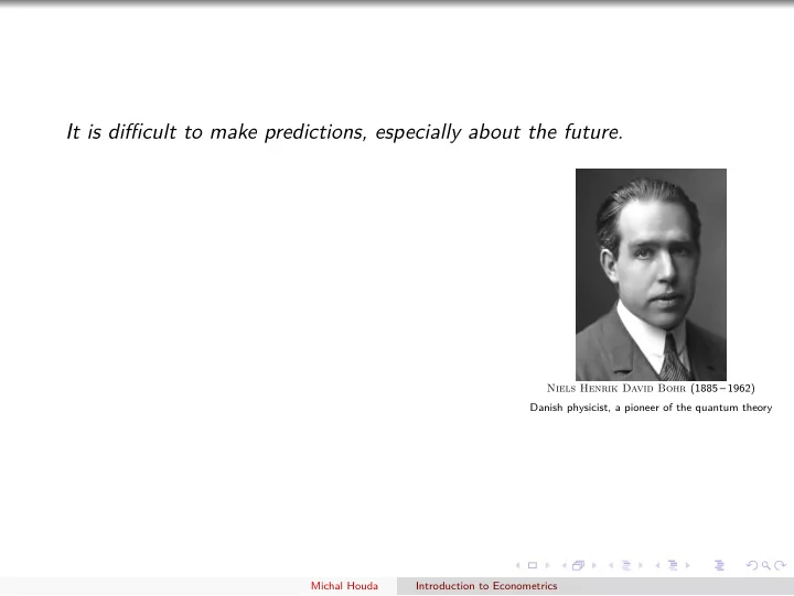
It is difficult to make predictions, especially about the future.

Niels Henrik David Bohr (1885 – 1962) Danish physicist, a pioneer of the quantum theory Michal Houda Introduction to Econometrics

Introduction to Econometrics

Selected Topics Michal Houda

University of South Bohemia in České Budějovice Department of Applied Mathematics and Informatics

Econometric Seminar, České Budějovice April 4, 2014

Michal Houda Introduction to Econometrics

Econometrics Econometrics

What Is Econometrics?

Michal Houda Introduction to Econometrics

What Is Econometrics

economic theory qualitative analysis economic relationships microeconomics, macroeconomics

Example: how the wage, inflation rate, unemployment, production, etc. are related

Michal Houda Introduction to Econometrics

What Is Econometrics

Michal Houda Introduction to Econometrics

What Is Econometrics

Economic Statistics

measuring, numerical expression of economic quantities quantitative analysis

Example: the price of fuel has augmented by 1,50 € last month

Michal Houda Introduction to Econometrics

What Is Econometrics

Michal Houda Introduction to Econometrics

What Is Econometrics

Mathematical Economics

mathematical models for example, (systems of) mathematical equations

Michal Houda Introduction to Econometrics

What Is Econometrics

Example Economic theory: household expenditures on a certain product of long-term consumption depends (somehow) on the total household expenditures, and on the price of the product Mathematical Economics: formulates the hypothesis by a mathematical model LE = a · TE + b · P where

LE . . . long-term household expenditures on the selected product TC . . . total household expenditures P . . . price of the product a, b . . . unknown parameters

Michal Houda Introduction to Econometrics

What Is Econometrics

Michal Houda Introduction to Econometrics

What Is Econometrics

Mathematical Statistics

mathematical modelling of different relationships between variables “mathematically” defines the measurement and investigates the methodology of this measurement

Michal Houda Introduction to Econometrics

What Is Econometrics

Example LE = a · TE + b · P Let

t = 1, . . . ,10 years . . . time, time intervals εt . . . error, disturbance, residuum, “remainings” in tth year

Statistical (econometric) model of the problem: LEt = a · TEt + b · Pt + εt ∀t Mathematical statistics provides methods to discover (estimate) the unknown parameters a and b.

Michal Houda Introduction to Econometrics

What Is Econometrics

Michal Houda Introduction to Econometrics

What Is Econometrics

Econometrics

linking economics, mathematics, and statistics discipline that using mathematical models, statistical methods, and empirical data (given by measurements or observations) verifies the conclusions of the economic theory

• r try to discover such relationships

Michal Houda Introduction to Econometrics

Econometric model

Econometric model LEt = a · TEt + b · Pt + εt ∀t created by a mathematical (statistical) formulation of a certain economic hypotheses if we have data:

year (t) 1 2 3 4 5 6 7 8 9 10 long-term exp. (LEt ) 3 4 5 6 7 8 9 10 12 14 total exp. (TEt ) 15 20 30 42 50 54 65 72 85 90 price (Pt ) 10 10 10 7 7 7 6 5 6 4 we can, by different (statistical, econometric) methods, for example, by the least squares method (OLS):

min → ε2

t

estimate parameters a and b of the model, and detect some other information about the quality of this estimate (on the computer: a = 0,14 and b = 0,08, and we have also found that b is not statistically significant, that is, the dependency of long-term expenditures LE on the price P is negligible)

Michal Houda Introduction to Econometrics

Differences from Related Disciplines

1

the data are not experimental, but observational (retrospective), usually random

2

the model assumptions set by the “nature” (not by the researcher), or they are not always fulfilled

3

the simplifications commonly used (and a correct interpretation of results is necessary). Five Steps in Empirical Analysis

1

qualitative analysis of the problem ⇒ economic model

2

mathematical/statistical transformation ⇒ econometric model

3

data ⇒ quantitative (empirical) analysis of the problem

4

economical/statistical verification of the model ⇒ testing the hypothesis

5

implementation/further exploration of the model

Michal Houda Introduction to Econometrics

The Structure of Economic Data

1

cross-sectional data

a set of objects (individuals, households, firms, cities, . . . ) taken at a given point in time usually obtained by random sampling

• rdering of the data is not important

2

time series data

• bservation of variables over time

chronological ordering potentially important information issues: (serial) dependence, seasonal patterns, . . .

3

pooled cross sections

cross-sectional data taken over time new sample taken at each time

4

panel (longitudinal) data

dtto, but time series for each cross-sectional object

Michal Houda Introduction to Econometrics

The Question of Causality

economist’s goal: establish a causal effect between variables, under ceteris paribus = “other (relevant) factors being equal” not easy task

number of affecting factors may be immense some of them cannot be held “fixed” in practice (e. g. education, experience) have we chosen enough factors to be held “fixed”

Econometrics: how to simulate a ceteris paribus experiment to estimate the causality of variables in question

Michal Houda Introduction to Econometrics

Definition of the Simple Linear Regression (SLR) Model

“explaining y in terms of of x” y = β0 + β1x + ε (1) y x ε dependent variable independent variable error term explained variable explanatory variable disturbance response variable control variable unobserved (other) factors predicted variable predictor variable residual term regressand regressor (covariate) Convention Y , X . . . random variable representing regressand, regressors (in econometrics often also written as y, x) y, x . . . observed (e. g. measured) values of Y , X ˆ y . . . calculated or predicted values of regressand ε . . . (non-observed) error or disturbance ˆ ε . . . calculated residuals

Michal Houda Introduction to Econometrics

Definition of the Simple Linear Regression Model

Linearity and Issues

Linearity: the effect of x on y is linear – if ∆ǫ = 0 then ∆y = β1∆x,

• i. e.

β1 = ∆y ∆x β1 . . . slope parameter β0 . . . intercept parameter Issues

1

the relationship never exact

2

the functional relationship may not be linear

3

how we can be sure to capture a ceteris paribus relationship between y and x

β1 measures the effect of x on y, other factors ε held fixed but, in fact, we ignore all these factors

⇒ we only get (more or less) reliable estimators of β0, β1, based on random sample under some (restrictive) assumption.

Michal Houda Introduction to Econometrics

Deriving the Ordinary Least Squares Estimates

Least Squares Method

Under zero conditional mean assumption (see later): E[y|x] = β0 + β1x . . . population regression function (PRF) Least Squares Method: min → SSR :=

n

• t=1

ˆ ε2

t = n

• t=1
• yt − (ˆ

β0 + ˆ β1xt)2 By deriving & setting the derivatives = 0, we obtain ˆ β1 = sample cov(x, y) sample var x =

• (xt − ¯

x)(yt − ¯ y)

• (xt − ¯

x)2 , ˆ β0 = ¯ y − ˆ β1¯ x ˆ y = ˆ β0 + ˆ β1x (2) . . . OLS regression line / sample regression function (SRF)

Michal Houda Introduction to Econometrics

Statistical Properties of the OLS Estimators

Assumptions for Simple Linear Regression

Assumption SLR 1 (Linearity in parameters) In the population model, y is related to x and ε as y = β0 + β1x + ε (3) Assumption SLR 2 (Random Sampling) We have the random sample (x1; y1), . . . , (xn; yn) from the population model given by (7). Assumption SLR 3 (Sample Variation in the Explanatory Variable) The sample outcomes on x (namely {xt, t = 1, . . . , n }) are not of the same value. Assumption SLR 4 (Zero Conditional Mean) E[ε|x] = 0

Michal Houda Introduction to Econometrics

Statistical Properties of the OLS Estimators

Unbiasedness of OLS

Theorem 1 (Unbiasedness of OLS) Under SLR.1–4, Eˆ β0 = β0 and Eˆ β1 = β1 for any values of β0, β1. In other words, ˆ β0 is unbiased estimator of β0 and ˆ β1 is unbiased estimator of β1. Remarks

1

Unbiasedness is the property of sampling, not of the sample

if the sample is typical, we obtain good estimators, but not always, we are so “lucky”, and we never know if we are lucky

2

Unbiasedness fails if any of SLR’s assumptions fails

the model is not (technically) linear (SLR.1) the data are time series with serial correlation, or the sample is not representative (SLR.2) if SLR.3 fails we cannot even obtain OLS estimators if SLR.4 fails the OLS estimators will probably be biased

Michal Houda Introduction to Econometrics

Statistical Properties of the OLS Estimators

Homoskedasticity

Assumption SLR 5 (Homoskedasticity) var[ε|x] = var[ε] =: σ2 > 0 compare with SLR.4 (not the same thing!) not needed for unbiasedness if ε and x are independent then SLR.4 and SLR.5 are fulfilled (this is a strong assumption) σ2 . . . error (disturbance) variance If SLR.5 fails ⇒ heteroskedasticity

Michal Houda Introduction to Econometrics

Statistical Properties of the OLS Estimators

Sampling Variance of the OLS Estimators

Theorem 2 (Sampling Variance of the OLS Estimators) Under SLR.1–5, var[ˆ β1|x1, . . . , xn] = σ2 SST x var[ˆ β0|x1, . . . , xn] = σ2 SST x · 1 n

• t

x 2

t

larger σ2, larger the variance of the slope estimate larger the variability in x, smaller the variance of the slope estimate a larger n should increase the variability in x issue: σ2 unknown

ˆ σ2 = 1 n − 2

n

• t=1

ˆ ε2

t = SSR

n − 2 (4) Theorem 3 (Unbiased estimator of error variance) Under SLR.1–5, Eˆ σ2 = σ2, that is, ˆ σ2 is unbiased estimator of σ2.

Michal Houda Introduction to Econometrics

Statistical Properties of the OLS Estimators

Example

ˆ σ = √ ˆ σ2 . . . standard error of regression (SER)

• s. e. ˆ

β1 := sd ˆ β1 = ˆ σ √SST x . . . standard error of ˆ β1 Example 4 (Wage and Education) Data: WAGE1, n = 526 wage = β0 + β1educ + ε

wage . . . in dollars per hour educ . . . years of schooling

• wage = −0.90 + 0.54educ,

R2 ≈ 0.1648

Michal Houda Introduction to Econometrics

Incorporating Nonlinearities in Simple Linear Regression

Models with Elasticities

ln(wage) = β0 + β1educ + ε change in interpretation β1 . . . (constant) semi-elasticity of wage with respect to educ ln(wage) = β0 + β1 ln(educ) + ε β1 . . . (constant) elasticity of wage with respect to educ Model Dependent var. Independent var. Interpretation of β1 Level-level y x ∆y = β1∆x Level-log y ln x ∆y = (β1/100)%∆x Log-level ln y x %∆y = 100β1∆x Log-log ln y ln x %∆y = β1%∆x

Michal Houda Introduction to Econometrics

Multiple Linear Regression

Motivating Example

Example 5 wage = β0 + β1educ + β2exper + ε

β1 . . . of primary interest β2 . . . we control the experience (for being fixed)

Generally: Multiple Linear Regression (MLR) model y = β0 + β1x1 + β2x2 + . . . + βkxk + ε (5) OLS method: min SSR :=

n

• t=1

ˆ εt =

• t
• yt − ˆ

yt

2 =

• t
• yt − (ˆ

β0 + ˆ β1xt1 + . . . + ˆ βkxtk)2 Key assumption: zero conditional mean E[ε|x1, x2, . . . , xk] = 0

Michal Houda Introduction to Econometrics

Mechanics of Ordinary Least Squares

Interpreting the OLS Regression Equation

ˆ y = ˆ β0 + ˆ β1x1 + ˆ β2x2 ∆ˆ y = ˆ β1∆x1 + ˆ β2∆x2 ˆ β0 . . . predicted value of y given x1 = x2 = 0 ˆ β1 . . . partial ceteris paribus effect of x1 on y ˆ β1 . . . partial ceteris paribus effect of x2 on y Example 6 (Hourly Wage Equation) Data: WAGE1 ln(wage) = 0.284 + 0.092educ + 0.0041exper + 0.022tenure

ceteris paribus interpretation even the data have not been collected in ceteris paribus fashion interpretation valid if we change more variables simultaneously ∆ ln(wage) = 0.0041∆exper + 0.022∆tenure (holding ∆educ fixed).

Michal Houda Introduction to Econometrics

Mechanics of Ordinary Least Squares

A “Partialling Out” Interpretation of Multiple Regression

Consider the regression xt1 = δ0 + δ1xt2 + rt1 Get ˆ rt1 . . . OLS residuals

uncorrelated with xt2

ˆ β1 obtained by the regression of yt = β0 + β1ˆ rt1 + εt as ˆ β1 =

• t ˆ

rt1yt

• t ˆ

r 2

t1

this means: only the part of xt1 uncorrelated with xt2 is related to y (by ˆ β1) ⇒ ˆ β1 measures the sample relationship between y and x1, after x2 has been partialled (netted) out similarly for more dimensions

Michal Houda Introduction to Econometrics

Mechanics of Ordinary Least Squares

A “Partialling Out” Interpretation of Multiple Regression

Comparing MLR with SLR ˜ y = ˜ β0 + ˜ β1x1 ˆ y = ˆ β0 + ˆ β1x1 + ˆ β2x2 ˜ β1 = ˆ β1 + ˆ β2ˆ δ1 Two special cases: if

ˆ β2 = 0 (partial effect of x2 on ˆ y is zero), or ˆ δ1 = 0 (x1 uncorrelated with x2),

then ˜ β1 = ˆ β1. Example 7 (Determinants of College GPA)

• colGPA = 1.286 + 0.453hsGPA + 0.0094ACT
• colGPA = 1.415 + 0.482hsGPA

fairly small difference, because ˆ β2 small, even that sample corr(hsGPA, ACT) ≈ 0.346

Michal Houda Introduction to Econometrics

Mechanics of Ordinary Least Squares

Goodness-of-Fit and Regression through Origin

R2 = SSE SST = 1 − SSR SST =

• t(yt − ¯

y)(ˆ yt − ˆ yt)

• t(yt − ¯

y)2

• (

t ˆ

yt − ˆ yt)2 (6)

(squared) correlation coefficient between the actual yt and the fitted ˆ yt never decreases when another independent variable included into the regression ⇒ not a good tool to decide whether to add a new variable to the regression small R2: not (necessarily) means that the regression is useless; rather: hard to predict individual outcomes of y

Michal Houda Introduction to Econometrics

Mechanics of Ordinary Least Squares

Goodness-of-Fit and Regression through Origin

R2 = SSE SST = 1 − SSR SST =

• t(yt − ¯

y)(ˆ yt − ˆ yt)

• t(yt − ¯

y)2

• (

t ˆ

yt − ˆ yt)2 (6)

(squared) correlation coefficient between the actual yt and the fitted ˆ yt never decreases when another independent variable included into the regression ⇒ not a good tool to decide whether to add a new variable to the regression small R2: not (necessarily) means that the regression is useless; rather: hard to predict individual outcomes of y

Regression through Origin ˜ yt = ˜ β1x1 + ˜ β2x2 + . . . + ˜ βkxk Properties of OLS no longer valid!

residuals do not have a zero sample average ¯ y = ˆ y R2 can actually be negative (if defined by 1 − SSR

SST ); sometimes replaced by [corr(y, ˆ

y)]2 OLS estimators of the slope are biased if β0 = 0 actually!

Michal Houda Introduction to Econometrics

Statistical Properties of the OLS Estimators

Assumptions for Simple Linear Regression

Assumption MLR 1 (Linearity in parameters) The population model can be written as y = β0 + β1x1 + . . . + βkxk + ε (7) Assumption MLR 2 (Random Sampling) We have the random sample

• (xt1, . . . , xtk; yt), t = 1, . . . , n
• from the population

model given by (7). Assumption MLR 3 (No Perfect Collinearity) None of the independent variables is constant and there are no exact linear relationship among the independent variables.

technical assumption for ˆ β to be well defined, mathematically rank X = k + 1 not independence (only linear perfect correlation forbidden) also fails if n < k + 1

Michal Houda Introduction to Econometrics

Statistical Properties of the OLS Estimators

Assumptions for Simple Linear Regression and Unbiasedness of OLS

Assumption MLR 4 (Zero Conditional Mean) E[ε|x] = 0 MLR.4 fails if

functional relationship misspecified (e. g., forgotten xj 2 using level variable instead ln and vice versa

• mitting an important factor correlated with any of x1, . . . , xk

sometimes

if MLR.4 holds: x . . . exogenous explanatory variables if MLR.4 fails: x . . . endogenous explanatory variables

Michal Houda Introduction to Econometrics

Statistical Properties of the OLS Estimators

Assumptions for Simple Linear Regression and Unbiasedness of OLS

Assumption MLR 4 (Zero Conditional Mean) E[ε|x] = 0 MLR.4 fails if

functional relationship misspecified (e. g., forgotten xj 2 using level variable instead ln and vice versa

• mitting an important factor correlated with any of x1, . . . , xk

sometimes

if MLR.4 holds: x . . . exogenous explanatory variables if MLR.4 fails: x . . . endogenous explanatory variables

Theorem 8 (Unbiasedness of OLS) Under MLR.1–4, Eˆ βj = βj for all j = 0, 1, . . . , k and for any values of the population parameters β0, . . . , βk. In other words, ˆ βj are unbiased estimators of the population parameters βj.

Michal Houda Introduction to Econometrics

Statistical Properties of the OLS Estimators

Unbiasedness of OLS

• A. Overspecified model

including irrelevant variables into the regression y = β0 + β1x1 + β2x2 + β3x3 + ε where β3 = 0 no effect in terms of unbiasedness: E(y|x1, x2, x3) = E(y|x1, x2) = β0 + β1x1 + β2x2 hence just Eˆ β3 = β3 = 0. but, undesirable effect on the variance of the OLS estimates (see later).

Michal Houda Introduction to Econometrics

Statistical Properties of the OLS Estimators

Unbiasedness of OLS

• A. Overspecified model

including irrelevant variables into the regression y = β0 + β1x1 + β2x2 + β3x3 + ε where β3 = 0 no effect in terms of unbiasedness: E(y|x1, x2, x3) = E(y|x1, x2) = β0 + β1x1 + β2x2 hence just Eˆ β3 = β3 = 0. but, undesirable effect on the variance of the OLS estimates (see later).

• B. Omitted variable – simple case

true model y = β0 + β1x1 + β2x2 + ε estimated by ˜ y = ˜ β0 + ˜ β1x1 using x2 = δ0 + δ1x1 + r1 ⇒ ˜ β1 = ˆ β1 + ˆ β2˜ δ1, hence E˜ β1 = β1 + β2˜ δ1 ˆ β1 unbiased if β2 = 0, or ˜ δ1 = 0 (that is, corr(x1, x2) = 0). example — hourly wage equation: wage = 0.584 + 0.083educ (ability omitted) cannot say 0.083 > true β1 (only a single sample!) but this is “true” on average (across all possible samples).

Michal Houda Introduction to Econometrics

Statistical Properties of the OLS Estimators

The Variance of the OLS Estimates

Assumption MLR 5 (Homoskedasticity) var[ε|x1, . . . , xk] = σ2 > 0 Theorem 9 (Sampling Variance of the OLS Estimators) Under MLR.1–5, var[ˆ βj|x1, . . . , xn] = σ2 SST j(1 − R2

j )

where SSTj :=

t(xtj − ¯

xj)2 and R2

j is from regressing xj on all other x’s.

Three components of the OLS variances

1

σ2 — error variance

feature of the population; can be reduced by adding more variables to the regression

2

SST j — total sample variation in x

rarely possible to influence by choosing “right” x’s can be increased by increasing the sample size

3

R2

j — linear relationship between x’s

R2

j close to 1 . . . multicollinearity

reduced by dropping the variables from the regression

Michal Houda Introduction to Econometrics

Statistical Properties of the OLS Estimators

Variance in Misspecified Model

y = β0 + β1x1 + β2x2 + ε true model ˆ y = ˆ β0 + ˆ β1x1 + ˆ β2x2 “right” estimate ˜ y = ˜ β0 + ˜ β1x1 “wrong” estimate var ˆ β1 = σ2 SST 1(1 − R2

1) > var ˜

β1 = σ2 SST 1 unless x1, x2 uncorrelated

if β2 = 0 ⇒ ˆ β1 unbiased, ˜ β1 biased with smaller variance if β2 = 0 ⇒ ˆ β1, ˜ β1 both unbiased, ˜ β1 with smaller variance

⇒ “wrong model” preferred in terms of variance! BUT

bias in ˜ β1 dos not shrink with growing sample size var ˆ β1, var ˜ β1 both shrink with sample size

⇒ multicollinearity is less important issue as the sample size grows

Michal Houda Introduction to Econometrics

Multiple Regression Analysis – Statistical Inference

Classical Linear Model (CLM)

Assumption MLR 6 (Normality) ε ∼ N(0; σ2) and it is independent of x1, . . . , xk. Theorem 10 (Normal Sampling Distribution) Under MLR.1–6, ˆ βj ∼ N(βj, var ˆ βj). Corollary 11 (t Distribution for the standardized estimators) Under MLR.1–6, ˆ βj − βj

• s. e. ˆ

βj ∼ tn−k−1.

Statistical packages usually provide t-ratio t ˆ

βj := ˆ

βj/ s. e. ˆ βj automatically ⇒ tests

H0 : βj = 0 against HA : βj = 0 are straightforward.

Michal Houda Introduction to Econometrics

Multiple Regression Analysis – Statistical Inference

One-Sided Tests

H0 : βj = 0 against HA : βj > 0 Example 12 (Hourly Wage Equation)

• ln(wage) = 0.284 + 0.092educ + 0.0041exper + 0.022tenure

H0 : βexper = 0 against HA : βexper = 0 texper ≈ 0.0041/0.0017 ≈ 2.39 p-value = Pr{texper > 2.39} = 1 20.0171 = 0.0085 H0 rejected (even at 1%). But the estimated return of experience is not large: for example, additional 3 years of experience provides only 3 × 0.0041 = 1.23% increase of wages . . . statistical vs. economic significance.

Michal Houda Introduction to Econometrics

Multiple Regression Analysis – Statistical Inference

Tests against Other Alternatives

H0 : βj = aj against HA : βj 0 Example 13 (Campus Crime and Student Enrollement) Data: CAMPUS (FBI’s Uniform Crime Report for 1992, n = 97) ln(crime) = β0 + β1 ln(enroll) + ε

• ln(crime) = −6.63 + 1.27 ln(enroll)

H0 : βexper = 1 against HA : βexper > 1 (crime is of more problem on larger campuses) tln(enroll) ≈ (1.27 − 1)/0.11 ≈ 2.46 p-value = Pr{texper > 2.46} ≈ 0.0079 H0 rejected (at 1%). Warning: this analysis holds no other factor fixed ⇒ elasticity 1.27 is not

Michal Houda Introduction to Econometrics

Multiple Regression Analysis – Statistical Inference

Testing a Single Linear Combination of Parameters

Example 14 (Return to Education) ln(wage) = β0 + β1jc + β2univ + β3exper + ε

jc . . . # years attending a two-year college univ . . . # years attending a four-year college exper . . . # months in the workforce

H0 : β1 = β2 against HA : β1 < β2 Cannot simply use individual t statistics as s. e.(ˆ β1 − ˆ β2) = s. e. ˆ β1 − s. e. ˆ β2. By some technique, t =

ˆ β1− ˆ β2 s.e.( ˆ β1− ˆ β2) ≈ −1.48, p-value = 0.070

⇒ H0 is not rejected at 5% (it is rejected at 10%) — there is some, but not strong, evidence of the campus size on criminal activities.

Michal Houda Introduction to Econometrics

Multiple Regression Analysis – Statistical Inference

Testing Multiple Linear Restrictions: F test

Example 15 (Baseball Players’ Salaries) ln(salary) = β0 + β1years + β2gamesyr + β3bavg + β4hrunsyr + β5rbisyr + ε

salary . . . 1993 total salary years . . . # years in the league gamesyr . . . average # games played per year bavg . . . career batting average hrunsyr . . . # home runs per year rbisyr . . . runs batted in per year Estimate Std. Error t value Pr(>|t|) (Intercept) 1.119e+01 2.888e-01 38.752 < 2e-16 *** years 6.886e-02 1.211e-02 5.684 2.79e-08 *** gamesyr 1.255e-02 2.647e-03 4.742 3.09e-06 *** bavg 9.786e-04 1.104e-03 0.887 0.376 hrunsyr 1.443e-02 1.606e-02 0.899 0.369 rbisyr 1.077e-02 7.175e-03 1.500 0.134

H0 : β3 = β4 = β5 = 0 against HA : nonH0 . . . multiple (joint, three) exclusion restrictions

Michal Houda Introduction to Econometrics

Multiple Regression Analysis – Statistical Inference

Testing Multiple Linear Restrictions: F test

Example 15 (Baseball Players’ Salaries) ln(salary) = β0 + β1years + β2gamesyr + β3bavg + β4hrunsyr + β5rbisyr + ε H0 : β3 = β4 = β5 = 0 against HA : nonH0 . . . multiple (joint, three) exclusion restrictions Data: MLB1 (n = 353) Restricted model: ln(salary) = β0 + β1years + β2gamesyr + ε

Test statistics: F-ratio F := (SSRr − SSRur)/q SSRur/(n − k − 1) ∼ Fq,n−k−1 In the example, F ≈ 9.55, p-value ≈ 4.10−6 ⇒ H0 rejected. Note again that all the three t-statistics are insignificant! (Reason: corr(hrusyn, rbisyr) ≈ 0.89).

Overall significance test: H0 : x1 = . . . = xk = 0

H0 often rejected, even if R2 is small

• ccasionally, the overall F is the focus of a study (e. g., to test whether some variable is

predictable based on selected factors — cf. efficient markets hypothesis)

Michal Houda Introduction to Econometrics

Multiple Regression Analysis – Statistical Inference

Testing General Linear Restrictions: F test

Example 16 ln(price) = β0 + β1 ln(assess) + β2 ln(lotsize) + β3 ln(sqrtft) + β4 ln(bdrms) + ε

price . . . house price assess . . . the assessed housing value (before sold) lotsize . . . size of the lot (in feet) sqrft . . . square footage bdrms . . . number of bedrooms

Data: HPRICE1, n = 88

Estimate Std. Error t value Pr(>|t|) (Intercept) 0.263743 0.569665 0.463 0.645 log(assess) 1.043065 0.151446 6.887 1.01e-09 *** log(lotsize) 0.007438 0.038561 0.193 0.848 log(sqrft)

• 0.103238

0.138430

• 0.746

0.458 bdrms 0.033839 0.022098 1.531 0.129

Are the assessed housing prices of a rational valuation? H0 : β1 = 1, β2 = β3 = β4 = 0

Michal Houda Introduction to Econometrics

Multiple Regression Analysis – Statistical Inference

Testing General Linear Restrictions: F test

Example 16 ln(price) = β0 + β1 ln(assess) + β2 ln(lotsize) + β3 ln(sqrtft) + β4 ln(bdrms) + ε Are the assessed housing prices of a rational valuation? H0 : β1 = 1, β2 = β3 = β4 = 0 F ≈ 0.661, p-value≈ 0.62 ⇒ failed to reject H0. There is no evidence against rational valuation.

Michal Houda Introduction to Econometrics

Heteroskedasticity

Consequences of Heteroskedasticity for OLS

MLR.1–4 (without homoskedasticity assumption) ⇒

unbiasedness of ˆ βj consistency of ˆ βj, ˆ σ2 (hence R2)

MLR.5 (homoskedasticity) var(ε|x1, . . . , xk) = σ2 ⇒

estimators of var ˆ βj unbiased valid statistical inference (t, F, LM)

without MLR.5 (heteroskedasticity)

estimators of var ˆ βj biased t, F, LM tests do not work (nor the confidence intervals) OLS no longer BLUE (even not asymptotically efficient)

Michal Houda Introduction to Econometrics

Heteroskedasticity

Heteroskedasticity-Robust Inference after OLS Estimation

Assumption 1 Heteroskedasticity of unknown form. yt = β0 + β1xt + εt heteroskedasticity: var(εt|xt) = σ2

t (not constant)

OLS estimator: ˆ β1 = β1 +

• t(xt − ¯

x)εt

• t(xt − ¯

x)2 = β1 +

• t(xt − ¯

x)εt SST x it can be shown that var ˆ β1 =

• t(xt − ¯

x)2σ2

t

SST 2

x

(note the homoskedastic result for σ2

t = σ2).

Michal Houda Introduction to Econometrics

Heteroskedasticity

Heteroskedasticity-Robust Inference after OLS Estimation

var ˆ β1 =

• t(xt − ¯

x)2σ2

t

SST 2

x

White (1980) – estimates var ˆ β1 by

• var ˆ

β1 =

• t(xt − ¯

x)2ˆ ε2

t

SST 2

x

where ˆ εt are residuals form the (initial) regression of y on x. For multiple linear regression model:

• var ˆ

βj =

• t ˆ

r 2

tj ˆ

ε2

t

SST 2

j

where ˆ rtj are residuals form the regression of xj on all remaining x’s, and SST j is the sum of squared residuals from this regression.

• var ˆ

βj . . . (White/Huber/Eicker) heteroskedasticity-robust standard error of ˆ βj t, F, LM statistics updated accordingly.

Michal Houda Introduction to Econometrics

Heteroskedasticity

Heteroskedasticity-Robust Inference after OLS Estimation

Remarks robustified standard error my be higher or lower (usually higher)

• ften one obtain similar results with usual and robustified standard

errors — but this is not the rule knowing the values of standard errors, one cannot conclude on the presence

• f heteroskedasticity(!)

heteroskedastic standard error are valid only for larger samples (for small samples, t-ratios must not have t distribution) usual t-ratio has the exact t distribution (t-test is exact).

Michal Houda Introduction to Econometrics

Heteroskedasticity

Testing for Heteroskedasticity

many different tests for testing heteroskedasticity; the modern can even detect the shape Example: y = β0 + β1x1 + . . . + βkxk H0 : var(ε|x1, . . . , xk) = σ2 If H0 is false, Eε2 can be (a) function of x’s. For example, ε2 = δ0 + δ1x1 + . . . + δkxk + ν In this case, H0 : δ1 = . . . = δk = 0. To get a tractable F test, replace unknown ε2 with squared residuals ˆ ε2. Asymptotic (LM) version of the test is known as Breusch–Pagan (BP) test for heteroskedasticity. Other modifications of the test are often used (e. g., White test)

Michal Houda Introduction to Econometrics

Heteroskedasticity

Weighted Least Squares Estimation

Assumption 2 Heteroskedasticity known up to a multiplicative constant, i. e., var(ε|x) = σ2h(x) Example 17 sav t = β0 + β1inct + εt (8) var(εt|inct) = σ2inct (that is h(x) = x) (9) As E

• εt

√inct

2|inct

• = σ2, the equation

sav t √inct = β0 √inct + β1 √ inct + εt √inct can be estimated by the usual OLS method under MLR.1–5. Estimators obtained with estimated (instead of known) function h are called feasible generalized least squares (FGLS) estimator.

Michal Houda Introduction to Econometrics

Further Topics

Not Covered by This Presentation

Regression Analysis with Cross-Sectional Data

efficiency of OLS asymptotics (non-normal distributions, consistency, large sample inference) data scaling – Beta coefficients models with quadratic terms interactions nonnested submodels confidence and prediction intervals, residual analysis qualitative (dummy) variables, linear probability models (with or without interactions) missing data, nonrandom samples, outliers

Time Series Analysis

finite lag models, trends, seasonality stationarity, weakly dependent time series serial correlation

Other (Advanced) Topics

panel data methods instrumental variables, two-stage least squares simultaneous equations models logit, probit models, Poisson regression

• etc. . . .

Michal Houda Introduction to Econometrics