Inversion of dispersion curves program SVDDispCurve.m l. 36 / 37: - - PowerPoint PPT Presentation

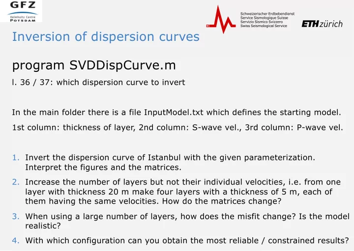
Inversion of dispersion curves program SVDDispCurve.m

• l. 36 / 37: which dispersion curve to invert

In the main folder there is a file InputModel.txt which defines the starting model. 1st column: thickness of layer, 2nd column: S-wave vel., 3rd column: P-wave vel.

• 1. Invert the dispersion curve of Istanbul with the given parameterization.

Interpret the figures and the matrices.

• 2. Increase the number of layers but not their individual velocities, i.e. from one

layer with thickness 20 m make four layers with a thickness of 5 m, each of them having the same velocities. How do the matrices change?

• 3. When using a large number of layers, how does the misfit change? Is the model

realistic?

• 4. With which configuration can you obtain the most reliable / constrained results?

Properties of the autocorrelation function program AutocorrFct_synth_1.m

• 1. Calculate the ACF of a simple sinusoid signal (f=0.16Hz). What do the various

plots show?

• 2. Add noise to the signal (l. 10-11), first a low level of noise, then a higher level
• f noise. How do the plots change? What does this mean?
• 3. For the noisy signal, use a filter (l. 14-16). First use a wide bandwidth, then use

a narrow bandwidth. What can you see?

• 4. Repeat all previous steps using two sinusoids with different frequencies and

amplitudes (change l. 18 in the code). What do you notice?

program ACF_noise.m

• 1. Test the influence of the filter for a real data set. Change both the filter

bandwidth and the frequency range. How do you interpret the velocity changes? For your info: Figure (88) shows the ACF for various time windows and the mean ACF, relative to which the velocity changes are calculated, in red.