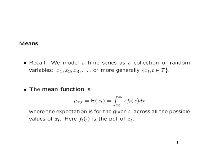
Means Recall: We model a time series as a collection of random - PowerPoint PPT Presentation

Means • Recall: We model a time series as a collection of random variables: x 1 , x 2 , x 3 , . . . , or more generally { x t , t ∈ T } . • The mean function is � ∞ µ x,t = E( x t ) = ∞ xf t ( x ) dx where the expectation is for the given t , across all the possible values of x t . Here f t ( · ) is the pdf of x t . 1

Example: Moving Average • w t is white noise, with E ( w t ) = 0 for all t • the moving average is v t = 1 � � w t − 1 + w t + w t +1 3 • so µ v,t = E ( v t ) = 1 � + E ( w t ) + E � � �� E � w t − 1 = 0 . w t +1 3 2

Moving Average Model with Mean Function 1 0 v −1 −2 0 100 200 300 400 500 Time 3

Example: Random Walk with Drift • The random walk with drift δ is t � x t = δt + w j j =1 • so t � � � µ x,t = E ( x t ) = δt + E w j = δt, j =1 a straight line with slope δ . 4

Random Walk Model with Mean Function 80 60 x 40 20 0 0 100 200 300 400 500 Time 5

Example: Signal Plus Noise • The “signal plus noise” model is x t = 2 cos(2 πt/ 50 + 0 . 6 π ) + w t • so µ x,t = E ( x t ) = 2 cos(2 πt/ 50 + 0 . 6 π ) + E ( w t ) = 2 cos(2 πt/ 50 + 0 . 6 π ) , the (cosine wave) signal. 6

Signal-Plus-Noise Model with Mean Function 4 2 x 0 −2 −4 0 100 200 300 400 500 Time 7

Covariances • The autocovariance function is, for all s and t , � � �� γ x ( s, t ) = E ( x s − µ x,s ) x t − µ x,t . • Symmetry: γ x ( s, t ) = γ x ( t, s ). • Smoothness: – if a series is smooth, nearby values will be very similar, hence the autocovariance will be large; – conversely, for a “choppy” series, even nearby values may be nearly uncorrelated. 8

Example: White Noise • If w t is white noise wn(0 , σ 2 w ), then  σ 2 w , s = t,  γ w ( s, t ) = E ( w s w t ) = 0 , s � = t.  • definitely choppy! 9

Autocovariances of White Noise gamma t s 10

Example: Moving Average • The moving average is v t = 1 � � w t − 1 + w t + w t +1 3 and E ( v t ) = 0, so γ v ( s, t ) = E ( v s v t ) = 1 �� � � �� 9E w s − 1 + w s + w s +1 w t − 1 + w t + w t +1  (3 / 9) σ 2 s = t w ,    (2 / 9) σ 2  w , s = t ± 1   = (1 / 9) σ 2 w , s = t ± 2     0 , otherwise .   11

Autocovariances of Moving Average gamma t s 12

Example: Random Walk • The random walk with zero drift is t � x t = w j j =1 and E ( x t ) = 0 • so γ x ( s, t ) = E ( x s x t )   s t � � = E w j w j   j =1 j =1 = min { s, t } σ 2 w . 13

Autocovariances of Random Walk gamma t s 14

• Notes: – For the first two models, γ x ( s, t ) depends on s and t only through | s − t | , but for the random walk γ x ( s, t ) depends on s and t separately. – For the first two models, the variance γ x ( t, t ) is constant, but for the random walk γ x ( t, t ) = tσ 2 w increases indefi- nitely as t increases. 15

Correlations • The autocorrelation function (ACF) is γ ( s, t ) ρ ( s, t ) = � γ ( s, s ) γ ( t, t ) • Measures the linear predictability of x t given only x s . • Like any correlation, − 1 ≤ ρ ( s, t ) ≤ 1. 16

Across Series • For a pair of time series x t and y t , the cross covariance function is � � �� γ x,y ( s, t ) = E ( x s − µ x,s ) y t − µ y,t . • The cross correlation function (CCF) is γ x,y ( s, t ) ρ x,y ( s, t ) = . � γ x ( s, s ) γ y ( t, t ) 17

Stationary Time Series • Basic idea: the statistical properties of the observations do not change over time. • Two specific forms: strong (or strict ) stationarity and weak stationarity. • A time series x t is strongly stationary if the joint distribution of every collection of values { x t 1 , x t 2 , . . . , x t k } is the same as that of the time-shifted values { x t 1 + h , x t 2 + h , . . . , x t k + h } , for every dimension k and shift h . • Strong stationarity is hard to verify. 18

If { x t } is strongly stationary, then for instance: • k = 1: the distribution of x t is the same as that of x t + h , for any h ; – in particular, if we take h = − t , the distribution of x t is the same as that of x 0 ; – that is, every x t has the same distribution; 19

• k = 2: the joint (bivariate) distribution of ( x s , x t ) is the same as that of ( x s + h , x t + h ), for any h ; – in particular, if we take h = − t , the joint distribution of ( x s , x t ) is the same as that of ( x s − t , x 0 ); – that is, the joint distribution of ( x s , x t ) depends on s and t only through s − t ; • and so on... 20

• A time series x t is weakly stationary if: – the mean function µ t is constant; that is, every x t has the same mean; – the autocovariance function γ ( s, t ) depends on s and t only through their difference | s − t | . • Weak stationarity depends only on the first and second mo- ment functions, so is also called second-order stationarity. • Strongly stationary (plus finite variance) ⇒ weakly stationary. • Weakly stationary �⇒ strongly stationary (unless some other property implies it, like normality of all joint distributions). 21

Simplifications � � • If x t is weakly stationary, cov depends on h but not x t + h , x t on t , so we write the autocovariances as � � γ ( h ) = cov x t + h , x t � � • Similarly corr x t + h , x t depends only on h , and can be written γ ( t + h, t ) = γ ( h ) ρ ( h ) = γ (0) . � γ ( t + h, t + h ) γ ( t, t ) 22

Examples • White noise is weakly stationary. • A moving average is weakly stationary. • A random walk is not weakly stationary. 23