Inverse problems for the study of climate-ecological processes in - PowerPoint PPT Presentation
Inverse problems for the study of climate-ecological processes in the conditions of anthropogenic impacts .. .. Report content: What are inverse problems? definitions differences from direct
Inverse problems for the study of climate-ecological processes in the conditions of anthropogenic impacts Пененко В.В. Цветова Е.А.
Report content: • What are inverse problems? • definitions • differences from direct problems • implementation specifics • How can we summarize the formulations of inverse problems? • variational approach • What is the meaning of the term climate-ecological? • How to take into account the different scales in climate & ecology? • How to consider and evaluate anthropogenic effects in inverse problems? • The main types of inverse problems on research topics 2
What are inverse problems? Direct problems are formulated as “In essence, the inverse of this task is the task in which the desired and the given are Initial- boundary- value problems. reversed” (Wikipedia, 1st grade of Goals defined; elementary school). • definitions What is known? • differences from The inverse problem is a type of tasks, often all model parameters; direct tasks arising in many sections of science, when sources of impact; • Specific the values of model parameters must be initial and boundary conditions. implementation: obtained from observable data. • Conditional well- Examples of inverse problems can be found posedness in the following areas: geophysics, Problems are solved “forward” in • Ill-posednes astronomy, medical imaging, computed time, they are mostly correct, • interrelated models tomography, remote sensing of the Earth, sometimes conditionally correct. and observational spectral analysis, scattering theory and non- data destructive testing tasks, etc. 3
What is the meaning of the term climate-ecological problems in the Earth system? • Earth system climate • Man • climatic zones of the globe • regional climate • Environment • climate of urban • Ecology agglomerations • meso-climate • microclimate 4
Features of mathematical modeling in environmental protection problems • The need to obtain and refine the • Nonlinearity, a variety of time forecast as measurement data scales and processes, high (up to becomes available . 1012) dimension of the considered Real time models operation Main pollutants: • Ozone (O3), carbon monoxide (CO), ammonia (NH3), hydrogen sulfide (H2S), sulfur The dioxide (SO2), nitrogen oxides (NO, NO2), formaldehyde difficulty (HCHO), ... of direct • Aerosols: PM 10, PM 2.5, nano modeling ... • radioactive ... High • biologically active ... uncertainty The uniqueness of • Unknown sources of impacts, initial and boundary conditions, rates of each situation transformations and other parameters of models, structure of models. • Lack of required measurement data 5
How can we present formulations of direct and inverse problems in a generalized form? Variational principle Formulation with weak constraints, combining • mathematical models of processes (in the form of an integral identity); • available observational data; • target (goal) functionals. For unification, we use • the classical method of Lagrange multipliers (1762); • adjoint functions • the concept of adjoint integrating factors 6
General structure of modeling systems L X L ( U Y f r , , , ) G ( U Y , ) f r 0 t 0 0 t 0 a The vector of functional arguments of the modeling system X U Y,f,r,ξ , Results and models of observations % H ( ) , m 1, M m m m Target functionals of studies ( ) F ( ) ( , ) x t dDdt ( F , ) , k 1, K . k k k k k D t D 7 t
Variational principle for combining all objects of the modeling system Integral identity * * I X φ , L X ,φ * G ( U Y , ) f r φ , dDdt 0 t D t X I , 0 system energy balance equation * * ( φ Q D ) adjoint functions vector t 8
Adjoint functions 1. "Global": Distributed Lagrange multipliers for combining process models, observational data, and prediction target functionals within a variational principle; 2. "Local": In the modeling technology in the decomposition and splitting mode in combination with the methods of finite elements / volumes: Solutions of homogeneous adjoint problems for the construction of numerical schemes with conservation laws (adjoint integrating factors) 9
System of convection-diffusion-reaction equations in models of hydrothermodynamics and atmospheric chemistry L ( ) X i div u div grad S ( ) φ ( f r ) 0, i 1, n i i i i t i i S ( ) φ P ( ) φ ( ), φ i 1, n i i i i 10
Extended functional of the variational principle with weak constraints ( r 0) h * h * ( , X , ) η I ( , X ) h D t h h h 0.5 ( W r r , ) ( W ξ ξ , ) 0.5 ( W ) ( ) 2 2 h 3 3 h 1 1 m 4 k D D D t t 11
Decomposition and splitting for the construction of numerical schemes and algorithms with the properties of the total approximation q q φ φ ; G ( U Y , ) φ ; t t 1 1 q q q f f ; r r ; 1; t t t j j 1 1 1 1 φ φ f r 0 ; 1, q t q q j j j 1 j 1 j 1 j 1 φ φ ; φ φ ; r r 1 1 12
Gateaux-variations for functionals. Algorithms for sensitivity relations S ( ), * S X φ , Definition of Gateaux derivatives for the functional p p ( S ) S S , p 1 p 0 Taylor series S 0 at For each structure of vectors p p S S S O , p 1 ! 1 When p = 1: Euler-Lagrange equations: systems of basic and adjoint equations, equations for uncertainties; sensitivity relations for target functionals to parameter variations When p = 2: sensitivity ratios of the second order; Hessian 13
Variations of extended functional ( p=1) % % % h h h % h * k k k (,..., ) , φ , φ , r k * φ φ r % % % % h h h h k k k k , ξ , Ψ , Y , U m ξ Ψ Y U m Stationarity conditions Sensitivity relations % h % h k , Y % h % h % h % h k Y k 0, k 0, k 0, k 0 φ φ r ξ * % h % h k , U k U 14
Basic algorithm for forward / inverse modeling % h h k φ G ( φ U Y ) - f - r , , 0 direct problem t φ % h T T k ( ) φ A ( φ U Y φ , , ) d 0, adjoint problem t k k k φ φ ( ) x 0, x D h T d ( ( φ ) 0.5 ( M )), k t t k k 1 1 φ 0 0 1 φ φ M φ ( x , 0 ), t 0 , Initial data with uncertainty a 3 k 1 * model uncertainty function r x ( , t ) M φ ( x , t ), 2 k h A ( φ U Y , , ) φ G ( φ φ U Y , , ) , 0 � � � approximation of time derivatives 15
Modeling technology based on variational principle Five fundamental spaces for environmental forecasting and design: • State functions of the direct problem • Solutions of adjoint problems • Uncertainty functions of process models • Sensitivity functions of process models and target functionals to variations of model parameters, initial data, functions of boundary conditions and sources of impacts • Sensitivity functions of target functionals to variations in observational data 16
Recommend
More recommend
Explore More Topics
Stay informed with curated content and fresh updates.
