Introduction to Support Vector Machines Starting from slides drawn - PowerPoint PPT Presentation
0. Introduction to Support Vector Machines Starting from slides drawn by Ming-Hsuan Yang and Antoine Cornu ejols SVM Bibliography 1. B. Boser, I. Guyon, V. Vapnik, A training algorithm for optimal margin classifier, 1992 C. Cortes,
0. Introduction to Support Vector Machines Starting from slides drawn by Ming-Hsuan Yang and Antoine Cornu´ ejols
SVM Bibliography 1. B. Boser, I. Guyon, V. Vapnik, “A training algorithm for optimal margin classifier”, 1992 C. Cortes, V. Vapnik, “Support vector networks”. Journal of Machine Learning, 20, 1995. V. Vapnik. “The nature of statistical learning theory”. Springer Verlag, 1995. C. Burges, “A tutorial on support vector machines for pat- tern recognition”. Data Mining and Knowledge Descovery, 2(2):955-974, 1998. N. Cristianini, J. Shawe-Taylor, “Support Vector Machines and other kernel-based learning methods”. Cambridge University Press, 2000. Andrew Ng, “Support Vector Ma- chines”, Stanford University, CS229 Lecture Notes, Part V.
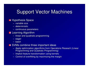
2. SVM — The Main Idea Given a set of data points which belong to either of two classes, find an optimal separating hyperplane - maximizing the distance (from closest points) of either class to the separating hyperplane, and - minimizing the risk of misclassifying the training samples and the unseen test samples. Approach: Formulate a constraint-based optimisation prob- lem, then solve it using quadratic programming (QP).
3. Optimal Separation Hyperplane maximal margin optimal separating hyperplane valid separating hyperplane
4. Plan 1. Linear SVMs The primal form and the dual form of linear SVMs Linear SVMs with soft margin 2. Non-Linear SVMs Kernel functions for SVMs An example of non-linear SVM
5. 1. Linear SVMs: Formalisation Let S be a set of points x i ∈ R d with i = 1 , . . . , m . Each point x i belongs to either of two classes, with label y i ∈ {− 1 , +1 } . The set S is linear separable if there are w ∈ R d and w 0 ∈ R such that y i ( w · x i + w 0 ) ≥ 1 i = 1 , . . ., m The pair ( w, w 0 ) defines the hyperplane of equation w · x + w 0 = 0 , named the separating hyperplane. The signed distance d i of a point x i to the separating hyper- plane ( w, w 0 ) is given by d i = w · x i + w 0 || w || . 1 1 It follows that y i d i ≥ || w || , therefore || w || is the lower bound on the distance between points x i and the separating hyper- plane ( w, w 0 ) .
6. Optimal Separating Hyperplane Given a linearly separable set S , the optimal separat- ing hyperplane is the separating hyperplane for which the distance to the closest (either positive or negative) 1 points in S is maximum, therefore it maximizes || w || .
7. geometric margin x i D(x) > 1 D(x) = 0 1 II w II D( ) x i support II w II vectors maximal margin w D(x) = 1 D(x) < −1 D(x) = −1 optimal separating hyperplane D ( x ) = w · x + w 0
8. Linear SVMs: The Primal Form 1 2 || w || 2 minimize subject to y i ( w · x i + w 0 ) ≥ 1 for i = 1 , . . . , m This is a constrained quadratic problem (QP) with d + 1 pa- rameters ( w ∈ R d and w 0 ∈ R ). It can be solved by quadratic optimisation methods if d is not very big ( 10 3 ). For large values of d ( 10 5 ): due to the Kuhn-Tucker theorem, since the above objective function and the associated con- straints are convex, we can use the method of Lagrange multipliers ( α i ≥ 0 , i = 1 , . . . , m ) to put the above problem under an equivalent “dual” form. Note: In the dual form, the variables ( α i ) will be subject to much simpler constraints than the variables ( w, w 0 ) in the primal form.
9. Linear SVMs: Getting the Dual Form The Lagrangean function associated to the primal form of the given QP is m L P ( w, w 0 , α ) = 1 2 || w 2 || − � α i ( y i ( w · x i + w 0 ) − 1) i =1 with α i ≥ 0 , i = 1 , . . . , m . Finding the minimum of L P implies m ∂L P � = − y i α i = 0 ∂w 0 i =1 m m ∂L P � � ∂w = w − y i α i x i = 0 ⇒ w = y i α i x i i =1 i =1 where ∂L P ∂w = ( ∂L P , . . . , ∂L P ) ∂w 1 ∂w d By substituting these constraints into L P we get its dual form m m m α i − 1 � � � L D ( α ) = α i α j y i y j x i · x j 2 i =1 i =1 j =1
10. Linear SVMs: The Dual Form i =1 α i − 1 � m � m � m j =1 α i α j y i y j x i · x j maximize i =1 2 � m i =1 y i α i = 0 subject to α i ≥ 0 , i = 1 , . . ., m The link between the primal and the dual form: The optimal solution ( w, w 0 ) of the primal QP problem is given by m � w = α i y i x i i =1 α i ( y i ( w · x i + w 0 ) − 1) = 0 for any i = 1 , . . ., m where α i are the optimal solutions of the above (dual form) optimisation problem.
11. Support Vectors The only α i (solutions of the dual form of our QP problem) that can be nonzero are those for which the constraints y i ( w · x i + w 0 ) ≥ 1 for i = 1 , . . ., m in the primal form of the QP are satisfied with the equality sign. Because most α i are null, the vector w is a linear combination of a relative small percentage of the points x i . These points are called support vectors because they are the closest points to the optimal separating hyperplane (OSH) and the only points of S needed to determine the OSH. The problem of classifying a new data point x is now simply solved by looking at sign ( w · x + w 0 ) .
12. Linear SVMs with Soft Margin If the set S is not linearly separable — or one simply ignores whether or not S is linearly separable —, the previous analysis can be generalised by introducing m non-negative (“slack”) variables ξ i , for i = 1 , . . ., m such that y i ( w · x i + w 0 ) ≥ 1 − ξ i , for i = 1 , . . . , m Purpose: to allow for a small number of missclassified points, for better generalisation or computational efficiency.
13. Generalised OSH The generalised OSH is then viewed as the solution to the problem: 2 || w || 2 + C 1 � m minimize i =1 ξ i subject to y i ( w · x i + w 0 ) ≥ 1 − ξ i for i = 1 , . . . , m ξ i ≥ 0 for i = 1 , . . . , m The associated dual form: i =1 α i − 1 � m � m � m j =1 α i α j y i y j x i · x j maximize i =1 2 � m subject to i =1 y i α i = 0 0 ≤ α i ≤ C, i = 1 , . . . , m As before: w = � m i =1 α i y i x i α i ( y i ( w · x i + w 0 ) − 1 + ξ i ) = 0 ( C − α i ) ξ i = 0
14. The role of C : it acts as a regularizing parameter: • large C ⇒ minimize the number of misclassified points 1 • small C ⇒ maximize the minimum distance || w ||
15. 2. Nonlinear Support Vector Machines • Note that the only way the data points appear in (the dual form of) the training problem is in the form of dot products x i · x j . • In a higher dimensional space, it is very likely that a linear separator can be constructed. • We map the data points from the input space R d into some space of higher dimension R n ( n > d ) using a function Φ : R d → R n • Then the training algorithm would depend only on dot products of the form Φ( x i ) · Φ( x j ) . • Constructing (via Φ ) a separating hyperplane with maximum margin in the higher-dimensional space yields a nonlinear decision boundary in the input space.
16. General Schema for Nonlinear SVMs Φ y h x Input Output space space Internal redescription space
17. Introducing Kernel Functions • But the dot product is computationally expensive... • If there were a “kernel function” K such that K ( x i , x j ) = Φ( x i ) · Φ( x j ) , we would only use K in the training algorithm. • All the previous derivations in the model of linear SVM hold (substituting the dot product with the kernel func- tion), since we are still doing a linear separation, but in a different space. • Important remark: By the use of the kernel function, it is possible to compute the separating hyperplane without explicitly carrying out the map into the higher space.
18. Some Classes of Kernel Functions for SVMs • Polynomial: K ( x, x ′ ) = ( x · x ′ + c ) q • RBF (radial basis function): K ( x, x ′ ) = e − || x − x ′|| 2 2 σ 2 • Sigmoide: K ( x, x ′ ) = tanh ( αx · x ′ − b )
19. An Illustration (a) (b) Decision surface ( a ) by a polynomial classifier, and ( b ) by a RBF. Support vectors are indicated in dark fill.
20. Important Remark The kernel functions require calculations in x ( ∈ R d ) , therefore they are not difficult to compute. It remains to determine which kernel function K can be as- sociated with a given (redescription space) function Φ . In practice, one proceeds vice versa: we test kernel functions about which we know that they correspond to the dot product in a certain space (which will work as redescription space, never made explicit). Therefore, the user operates by “trial and error”... Advantage: the only parameters when training an SVM are the kernel function K , and the “tradeoff” parameter C .
21. Mercer’s Theorem (1909): A Characterisation of Kernel Functions for SVMs Theorem: Let K : R d × R d → R be a symmetrical function. K represents a dot product, i.e. there is a function Φ : R d → R n such that K ( x, x ′ ) = Φ( x ) · Φ( x ′ ) if and only if K ( x, x ′ ) f ( x ) f ( x ′ ) dx dx ′ ≥ 0 � � f 2 ( x ) dx is finite. for any function f such that Remark: The theorem doesn’t say how to construct Φ .
22. Some simple rules for building (Mercer) kernels If K 1 and K 2 are kernels over X × X , with X ⊆ R n , then • K ( x, y ) = K 1 ( x, y ) + K 2 ( x, y ) • K ( x, y ) = aK 1 ( x, y ) , with a ∈ R + • K ( x, y ) = K 1 ( x, y ) K 2 ( x, y ) are also kernels.
Recommend
More recommend
Explore More Topics
Stay informed with curated content and fresh updates.
