Chapter IX: Classification* 1. Basic idea 2. Decision trees 3. - PowerPoint PPT Presentation
Chapter IX: Classification* 1. Basic idea 2. Decision trees 3. Nave Bayes classifier 4. Support vector machines 5. Ensemble methods * Zaki & Meira: Ch. 18, 19, 21, 22; Tan, Steinbach & Kumar: Ch. 4, 5.35.6 IR&DM 13/14 16
Chapter IX: Classification* 1. Basic idea 2. Decision trees 3. Naïve Bayes classifier 4. Support vector machines 5. Ensemble methods * Zaki & Meira: Ch. 18, 19, 21, 22; Tan, Steinbach & Kumar: Ch. 4, 5.3–5.6 IR&DM ’13/14 16 January 2014 IX.4&5- 1
IX.4 Support vector machines* 1. Basic idea 2. Linear, separable SVM 2.1. Lagrange multipliers 3. Linear, non-separable SVM 4. Non-linear SVM 4.1. Kernel method * Zaki & Meira: Ch. 5 & 21; Tan, Steinbach & Kumar: Ch. 5.5; Bishop: Ch. 7.1 IR&DM ’13/14 16 January 2014 IX.4&5- 2
Basic idea B 1 B 1 Which one is better? There are many possible answers B 2 B 2 B 2 How do you define ”better”? Find a linear hyperplane (decision boundary) that will separate the • • • • • classes • IR&DM ’13/14 16 January 2014 IX.4&5- 3
Formal definitions • Let class labels be –1 and 1 • Let classification function f be a linear function: f ( x ) = w T x + b – Here w and b are the parameters of the classifier – The class of x is sign( f ( x )) – The distance of x to the hyperplane is | f ( x )|/|| w || • The decision boundary of f is the hyperplane z for which f ( z ) = w T z + b = 0 • The quality of the classifier is based on its margin IR&DM ’13/14 16 January 2014 IX.4&5- 4
The margin B 1 has bigger margin ⇒ it is better B 1 The margin is twice the length of the shortest vector perpendicular to the decision boundary B 2 from the decision boundary to a data b 21 point. b 22 margin b 11 b 12 • IR&DM ’13/14 16 January 2014 IX.4&5- 5
The margin in math B 1 • Around B i we have two parallel hyperplanes b i 1 and b i 2 B 2 b 21 – Scale w and b s.t. b 22 b i 1 : w T z + b = 1 b i 2 : w T z + b = –1 margin b 11 • Let x 1 be in b i 1 and x 2 be in b 12 b i 2 • – The margin d is the distance from x 1 to the hyperplane plus the distance from x 2 to the hyperplane: d = 2/|| w || This is what we want to maximize! IR&DM ’13/14 16 January 2014 IX.4&5- 6
Linear, separable SVM • Given the data, we want to find w and b s.t. – w T x i + b ≥ 1 if y i = 1 – w T x i + b ≤ –1 if y i = –1 • In addition, we want to maximize the margin – Equals to minimizing f ( w ) = || w || 2 /2 Linear, separable SVM. min w || w || 2 /2 subject to y i ( w T x i + b ) ≥ 1, i = 1, …, N IR&DM ’13/14 16 January 2014 IX.4&5- 7
Intermezzo: Lagrange multipliers • A method to find extrema of constrained functions via derivation • Problem: minimize f ( x ) subject to g ( x ) = 0 – Without constraint we can just derive f (x) • But the extrema we obtain might be unfeasible given the constraints • Solution: introduce Lagrange multiplier λ – Minimize L ( x , λ ) = f ( x ) – λ g ( x ) – ∇ f ( x ) – λ ∇ g ( x ) = 0 • ∂ L / ∂ x i = ∂ f / ∂ x i – λ×∂ g / ∂ x i = 0 for all i • ∂ L / ∂λ = g ( x ) = 0 The constraint! IR&DM ’13/14 16 January 2014 IX.4&5- 8
More on Lagrange multipliers • For many constraints, we need to add one multiplier for each constraint – L ( x , λ ) = f ( x ) – Σ j λ j g j ( x ) – Function L is known as the Lagrangian • Minimizing the unconstrained Lagrangian equals minimizing the constrained f – But not all solutions to ∇ f ( x ) – Σ j λ j ∇ g j ( x ) = 0 are extrema – The solution is in the boundary of the constraint only if λ j ≠ 0 IR&DM ’13/14 16 January 2014 IX.4&5- 9
Example minimize f ( x , y ) = x 2 y subject to g ( x , y ) = x 2 + y 2 = 3 L ( x , y , λ ) = x 2 y + λ ( x 2 + y 2 – 3) ∂ L ∂ x = 2 xy + 2 λ x = 0 ∂ L ∂ y = x 2 + 2 λ y = 0 ∂ L ∂λ = x 2 + y 2 − 3 = 0 Solution: x = ± √ 2, y = –1 IR&DM ’13/14 16 January 2014 IX.4&5- 10
Karush–Kuhn–Tucker conditions • Lagrange multipliers can only handle equality constraints • Simple Karush–Kuhn–Tucker (KKT) conditions – g i (for all i ) are affine functions – λ i ≥ 0 for all i – λ i g i ( x ) = 0 for all i and locally optimum x • If KKT conditions are satisfied, then minimizing the Lagrangian minimizes f with inequality constraints IR&DM ’13/14 16 January 2014 IX.4&5- 11
Solving the linear, separable SVM Linear, separable SVM. min w || w || 2 /2 subject to y i ( w T x i + b ) ≥ 1, i = 1, …, N N L p = 1 Primal 2 k w k 2 − X y i ( w T x i + b ) − 1 � � λ i Lagrangian i = 1 N ∂ L p X λ i y i x i ∂ w = 0 ⇒ w = w is a linear combination of x i s i = 1 N ∂ L p X Signed Lagrangians have to sum to 0 λ i y i = 0 ∂ b = 0 ⇒ i = 1 λ i > 0 KKT conditions for λ i y i ( w T x i + b ) − 1 � � = 0 λ i IR&DM ’13/14 16 January 2014 IX.4&5- 12
From primal to dual to get λ i substitute N ∂ L p X ∂ w = 0 ⇒ w = λ i y i x i N L p = 1 i = 1 2 k w k 2 − X y i ( w T x i + b ) − 1 � � λ i N ∂ L p i = 1 X λ i y i = 0 ∂ b = 0 ⇒ i = 1 N N N λ i − 1 Dual X X X λ i λ j y i y j x T L d = i x j Lagrangian 2 c i t a e i = 1 i = 1 j = 1 r r a d a s u d q o h d r t a e m s Quadratic on λ i ’s Training data d i n h n a t o t e S i v t a l o z s i m o t Linear, separable SVM, dual form. i t d p e o s u max λ L d = ∑ i λ i – 1/2 ∑ i,j λ i λ j y i y j x iT x j subject to λ i ≥ 0, i = 1, …, N IR&DM ’13/14 16 January 2014 IX.4&5- 13
Getting the rest… • After solving λ i ’s, we can substitute to get w and b w = P N – i = 1 λ i y i x i – For b , by KKT we have λ i ( y i ( w T x i + b ) – 1) = 0 – We get one b i for each non-zero λ i • Due to numerical problems b i ’s might not be the same ⇒ take the average • With this, we can now classify unseen entries x by sign( w T x + b ) IR&DM ’13/14 16 January 2014 IX.4&5- 14
Excuse me sir, but why… • …is it called support vector machine? • Most λ i ’s will be 0 • If λ i > 0, then y i ( w T x i + b ) = 1 ⇒ x i is in the margin hyperplane – These x i ’s are called support vectors • Support vectors define the decision boundary – Other have zero coefficients in the linear combination • Support vectors are the only things we care! IR&DM ’13/14 16 January 2014 IX.4&5- 15
The picture of a support vector B 1 A support vector And another B 2 b 21 b 22 margin b 11 b 12 • IR&DM ’13/14 16 January 2014 IX.4&5- 16
Linear, non-separable SVM • • What if the data is not linearly separable? f the problem is not linearly separabl IR&DM ’13/14 16 January 2014 IX.4&5- 17
The slack variables • Allow misclassification but pay for it • The cost is defined by slack variables ξ i > 0 – Change the optimization constraints to y i ( w T x i + b ) ≥ 1 – ξ i • If ξ i = 0, this is as before • If 0 < ξ i < 1, the point x i is correctly classified, but within the margin • If ξ i ≥ 1, the point is in the decision boundary or on the wrong side of it • We want to maximize the margin and minimize the slack variables IR&DM ’13/14 16 January 2014 IX.4&5- 18
Linear, non-separable SVM Linear, non-separable SVM. min w, ξ (|| w || 2 /2 + C ∑ i ( ξ i ) k ) subject to y i ( w T x i + b ) ≥ 1 – ξ i , i = 1, …, N ξ i ≥ 0, i = 1, …, N • Constants C and k define the cost of misclassification – If C = 0, no misclassification is allowed – If C → ∞ , width of margin doesn’t matter – k is typically either 1 or 2 • k = 1 is the hinge loss • k = 2 is the quadratic loss IR&DM ’13/14 16 January 2014 IX.4&5- 19
Lagrangian with slack variables and k = 1 • The Lagrange multipliers are λ i and µ i – λ i ( y i ( w T x i + b ) – 1 + ξ i ) = 0 with λ i ≥ 0 – µ i ( ξ i – 0) = 0 with µ i ≥ 0 • The primal Lagrangian is The objective function 2 k w k 2 + C P N – L p = 1 i = 1 ξ i − P N − P N � y i ( w T x i + b ) − 1 + ξ i � i = 1 λ i i = 1 µ i ξ i The constraints IR&DM ’13/14 16 January 2014 IX.4&5- 20
The dual } N N ∂ L p X X ∂ w = w − λ i y i x i = 0 ⇒ w = λ i y i x i i = 1 i = 1 substitute to N Partial ∂ L p Lagrangian X λ i y i = 0 ∂ b = − derivatives i = 1 ∂ L p = C − λ i − µ i = 0 ⇒ λ i + µ i = C ∂ξ i N N N Dual λ i − 1 X X X λ i λ j y i y j x T L D = i x j Lagrangian 2 i = 1 i = 1 j = 1 The same as before! Linear, non-separable SVM, dual form. max λ L d = ∑ i λ i – 1/2 ∑ i,j λ i λ j y i y j x iT x j subject to 0 ≤ λ i ≤ C , i = 1, …, N IR&DM ’13/14 16 January 2014 IX.4&5- 21
Weight vector and bias • Support vectors are again those with λ i > 0 – Support vector x i can be in margin or have positive slack ξ i • Weight vector w as before: w = ∑ i λ i y i x i • µ i = C – λ i ⇒ ( C – λ i ) ξ i = 0 – The support vectors that are in the margin are those where λ i = 0 ⇒ ξ i = 0 (as C > 0) – Therefore we can solve bias b as the average of b i ’s: b i = y i – w T x i IR&DM ’13/14 16 January 2014 IX.4&5- 22
Non-linear SVM (a.k.a. kernel SVM) What if the decision boundary is not linear? IR&DM ’13/14 16 January 2014 IX.4&5- 23
Transforming data Transform the data into higher-dimensional space (x 1 + x 2 ) 4 IR&DM ’13/14 16 January 2014 IX.4&5- 24
Recommend
More recommend
Explore More Topics
Stay informed with curated content and fresh updates.

![Classification Image Classification Set of predefined categories [eg: table, apple, dog, giraffe]](https://c.sambuz.com/743996/classification-s.webp)
